Section 5.9 Approximate Integration
Section 5.9 Approximate Integration. Practice HW from Stewart Textbook (not to hand in) p. 421 # 3 – 15 odd. Note: Many functions cannot be integrated using the basic integration formulas or with any technique of integration (substitution, parts, etc.).

Section 5.9 Approximate Integration
E N D
Presentation Transcript
Section 5.9 Approximate Integration Practice HW from Stewart Textbook (not to hand in) p. 421 # 3 – 15 odd
Note: Many functions cannot be integrated using the basic integration formulas or with any technique of integration (substitution, parts, etc.). Examples: , .
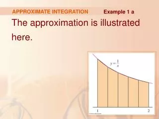
As a result, we cannot use the Fundamental Theorem of Calculus to determine the area under the curve. We must use numerical techniques. We have already seen how to do this using left, right, midpoint sums. In this section, we will examine two other techniques, which in general will produce more accuracy with less work, to approximate definite integrals.
Trapezoid Rule The idea behind the trapezoid rule is to approximate the area under a curve using the area of trapezoids. Suppose we have the following diagram of a trapezoid.
Recall that the area of the trapezoid is given by the following formula: Area of trapezoid = (base)(Average of the height)
Suppose we have a function which is continuous and bounded for . Suppose we desire to find the area A under the graph of f from x = a to x = b. To do this, we divide the interval for into n equal subintervals of width and form n trapezoids (subintervals) under the graph of f . Let be the endpoints of each of the subintervals.
Trapezoid Rule The definite integral of a continuous function f on the interval [a, b] can be approximated using n subintervals as follows: where , and .
Example 1: Use the trapezoid rule to approximate for n = 4 subintervals. Solution:
Simpson’s Rule Use’s a sequence of quadratic functions (parabolas) to approximate the definite integral. Theorem: Given a quadraticfunction then
We again partition the interval [a, b] into n equal subintervals of length . Note that n must be even. Here, we have , n is even.
On each double subinterval , we approximate the area under f by approximating the area under the polynomial p(x).
Similarly, , etc. Repeating this process for all subintervals, we get the following rule.
Simpson’s Rule Let f be continuous on [a, b]. For an even number of subintervals, where , and .
Example 2: Use Simpson’s rule to approximate for n = 4 subintervals. Solution:
Example 3: Use the trapezoidal and Simpson’s rule to approximate using n = 8 subintervals. Solution: (In typewritten notes)