6.4 Integration with tables and computer algebra systems 6.5 Approximate Integration

1. 6.4 Integration with tables and computer algebra systems6.5 Approximate Integration

2. Tables of Integrals • A table of 120 integrals, categorized by form, is provided on the References Pages at the back of the book. • References to more extensive tables are given in the textbook. • Integrals do not often occur in exactly the form listed in a table. • Usually we need to use the Substitution rule or algebraic manipulation to transform a given integral into one of the forms in the table. • Example: Evaluate • In the table we have forms involving • Let u = ln x. • Then using the integral #21 in the table,

3. Computer Algebra Systems (CAS) • Matlab, Mathematica, Maple. • CAS also can perform substitutions that transform a given integral into one that occurs in its stored formulas. • But a hand computation sometimes produces an indefinite integral in a form that is more convenient than a machine answer. • Example: Evaluate • Maple and Mathematica give the same answer: • If we integrate by hand instead, using the substitution u = x2 + 5, we get • This is a more convenient form of the answer.

4. Can we integrate all continuous functions? • Most of the functions that we have been dealing with are what are called elementary functions. These are the polynomials, rational functions, exponential functions, logarithmic functions, trigonometric and inverse trigonometric functions, and all functions that can be obtained from these by the five operations of addition, subtraction, multiplication, division, and composition. • If f is an elementary function, then f ’ is an elementary function, but its antiderivative need not be an elementary function. Example, In fact, the majority of elementary functions don’t have elementary antiderivatives. How to find definite integrals for those functions? Approximate!

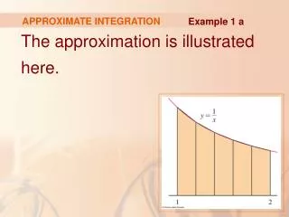
5. Approximating definite integrals:Riemann Sums Recall that the definite integral is defined as a limit of Riemann sums. A Riemann sum for the integral of a function f over the interval [a,b] is obtained by first dividing the interval [a,b] into subintervals and then placing a rectangle, as shown below, over each subinterval. The corresponding Riemann sum is the combined area of the green rectangles. The height of the rectangle over some given subinterval is the value of the function f at some point of the subinterval. This point can be chosen freely. Taking more division points or subintervals in the Riemann sums, the approximation of the area of the domain under the graph of f becomes better.

6. Approximating definite integrals:different choices for the sample points • Recall that where xi* is any point in the ith subinterval [xi-1,xi]. • If xi* is chosen to be the leftendpoint of the interval, then xi* = xi-1 and we have • If xi* is chosen to be the right endpoint of the interval, then xi* = xi and we have • Lnand Rn are called the left endpoint approximation and right endpoint approximation , respectively.

7. Example First find the exact value using definite integrals. Actual area under curve:

8. Approximate area: Left endpoint approximation: (too low)

9. Approximate area: Right endpoint approximation: (too high) Averaging the right and left endpoint approximations: (closer to the actual value)

10. Averaging the areas of the two rectangles is the same as taking the area of the trapezoid above the subinterval.

11. Trapezoidal rule This gives us a better approximation than either left or right rectangles.

12. Approximate area: Can also apply midpoint approximation: choose the midpoint of the subinterval as the sample point. The midpoint rule gives a closer approximation than the trapezoidal rule, but in the opposite direction.

13. Midpoint rule

14. Trapezoidal Rule: (higher than the exact value) 1.25% error Midpoint Rule: 0.625% error (lower than the exact value) Notice that the trapezoidal rule gives us an answer that has twice as much error as the midpoint rule, but in the opposite direction. If we use a weighted average: This is the exact answer!

15. twice midpoint trapezoidal This weighted approximation gives us a closer approximation than the midpoint or trapezoidal rules. Midpoint: Trapezoidal:

16. Simpson’s rule Simpson’s rule can also be interpreted as fitting parabolas to sections of the curve. Simpson’s rule will usually give a very good approximation with relatively few subintervals.

17. Example:

18. Error bounds for the approximation methods Examples of error estimations on the board.