Sliding Window Filters
Sliding Window Filters. Longin Jan Latecki latecki@temple.edu October 9, 2002. Linear Image Filters Linear operations calculate the resulting value in the output image pixel f(i,j) as a linear combination of brightness in a local neighborhood of the pixel h(i,j) in the input image.

Sliding Window Filters
E N D
Presentation Transcript
Sliding Window Filters Longin Jan Latecki latecki@temple.edu October 9, 2002
Linear Image Filters • Linear operations calculate the resulting value in the output image pixel f(i,j) as a linear combination of brightness in a local neighborhood of the pixel h(i,j) in the input image. • This equation is called to discrete convolution: Function w is called a convolution kernel or a filter mask. In our case it is a rectangle of size (2a+1)x(2b+1).
Exercise: Compute the 2-D linear convolution of the following two signal X with mask w. Extend the signal X with 0’s where needed.
Image smoothing = image blurring Averaging of brightness values is a special case of discrete convolution. For a 3 x 3 neighborhood the convolution mask w is • Applying this mask to an image results in smoothing. • Matlab example program is filterEx1.m • Local image smoothing can effectively eliminate impulsive noise or degradations appearing as thin stripes, but does not work if degradations are large blobs or thick stripes.
The significance of the central pixel may be increased to better reflect properties of Gaussian noise:
Edge detectors • locate sharp changes in the intensity function • edges are pixels where brightness changes abruptly. • Calculus describes changes of continuous functions using derivatives; an image function depends on two variables - partial derivatives. • A change of the image function can be described by a gradient that points in the direction of the largest growth of the image function. • An edge is a property attached to an individual pixel and is calculated from the image function behavior in a neighborhood of the pixel. • It is a vector variable: • magnitude of the gradient and direction
The gradient direction gives the direction of maximal growth of the function, e.g., from black (f(i,j)=0) to white (f(i,j)=255). • This is illustrated below; closed lines are lines of the same brightness. • The orientation 0° points East.
Edges are often used in image analysis for finding region boundaries. • Boundary and its parts (edges) are perpendicular to the direction of the gradient.
The gradient magnitude and gradient direction are continuous image functions, where arg(x,y) is the angle (in radians) from the x-axis to the point (x,y).
Sometimes we are interested only in edge magnitudes without regard to their orientations. • The Laplacian may be used. • The Laplacian has the same properties in all directions and is therefore invariant to rotation in the image. • The Laplace operator is a very popular operator approximating the second derivative which gives the gradient magnitude only.
The Laplacian is approximated in digital images by a convolution sum. • A 3 x 3 mask for 4-neighborhoods and 8-neighborhood • A Laplacian operator with stressed significance of the central pixel or its neighborhood is sometimes used. In this approximation it loses invariance to rotation
A digital image is discrete in nature, derivatives must be approximated by differences. • The first differences of the image g in the vertical direction (for fixed i) and in the horizontal direction (for fixed j) • n is a small integer, usually 1. The value n should be chosen small enough to provide a good approximation to the derivative, but large enough to neglect unimportant changes in the image function.
Gradient operators can be divided into three categories • I. Operators approximating derivatives of the image function using differences. • rotationally invariant (e.g., Laplacian) need one convolution mask only. Individual gradient operators that examine small local neighborhoods are in fact convolutions and can be expressed by convolution masks. • approximating first derivatives use several masks, the orientation is estimated on the basis of the best matching of several simple patterns. Operators which are able to detect edge direction. Each mask corresponds to a certain direction.
II. Operators based on the zero crossings of the image function second derivative (e.g., Marr-Hildreth or Canny edge detector). • III. Operators which attempt to match an image function to a parametric model of edges. Parametric models describe edges more precisely than simple edge magnitude and direction and are much more computationally intensive. • The categories II and III will not be covered here;
Roberts operator • The magnitude of the edge is computed as The primary disadvantage of the Roberts operator is its high sensitivity to noise, because very few pixels are used to approximate the gradient.
Prewitt operator • The Prewitt operator approximates the first derivative, similarly to the Sobel, Kirsch, Robinson and some other operators that follow. • Operators approximating first derivative of an image function are sometimes called compass operators because of the ability to determine gradient direction. • The gradient is estimated in eight (for a 3 x 3 convolution mask) possible directions. Larger masks are possible. • The direction of the gradient is given by the mask giving maximal response. This is valid for all following operators approximating the first derivative.
Sobel operator • Used as a simple detector of horizontality and verticality of edges in which case only masks h1 and h3 are used. • If the h1 response is y and the h3 response x, we might then derive edge strength (magnitude) as and direction as arctan (y / x). Matlab example program is filterEx1.m
Robinson operator Kirsch operator
Nonlinear Image Filters Median is an order filter, it uses order statistics. Given an NxN window W(x,y) with pixel (x,y) being the midpoint of W, the pixel intensity values of pixels in W are ordered from smallest to the largest, as follow: Median filter selects the middle value as the value of (x,y).
For comparison see Order Filters on http://www.ee.siue.edu/~cvip/CVIPtools_demos/mainframe.shtml Homework 2 Implement in Matlab a linear filter for image smoothing (blurring) and a nonlinear filters: median, opening, and closing. Apply them to noise_1.gif, noise_2.gif in http://www.cis.temple.edu/~latecki/CIS581-02/Images/ and to one example image of your choice. Compare the results.