Segmentation with raster sliding local window
270 likes | 470 Vues
Segmentation with raster sliding local window. Nelson Chang Institute of Electronics, National Chiao Tung University. Outline. Stereo Matching with Segment Traditional Watershed-based Segmentation Downfall of tradition segmentation methods Proposed Raster Sliding Local Window Method

Segmentation with raster sliding local window
E N D
Presentation Transcript
Segmentation with raster sliding local window Nelson Chang Institute of Electronics, National Chiao Tung University
Outline • Stereo Matching with Segment • Traditional Watershed-based Segmentation • Downfall of tradition segmentation methods • Proposed Raster Sliding Local Window Method • Result • Future work
Mean Shift vs. Watershed Watershed Mean Shift
Traditional Watershed-based Segmentation • Steps • Generate Gradient Map • Reconstruction/Global Denoise • Watershed flooding or Rain dropping • Region Merging
What makes an algorithm efficient to implement? state 0 state 0 state 3 • Regular • Simple control • High data reusability • Parallel • More scalable • Small storage • Lower cost • More fast memory usage state 1 state 1 state 2 state 2 state 4 Simple FSM Data reuse!!! PE PE PE PE PE PE 4x speed up!! PE PE Slow SDRAM Temporary Data Temporary Data Fast SRAM
Traditional Watershed and Topoggan Irregular jumpy access pattern HW: hard to reuse SW: low cache hit • Watershed Flooding • Bottom-up • Finds the minimum first
Traditional Watershed and Topoggan Irregular access start point HW: less chance to reuse SW: more cache miss More regular local access pattern than watershed • Topoggan Rain Dropping • Top-down • Finds the maximum peak first • Drop rain • Back trace the path Back trace water flow path (tree traversal) High data dependency HW: less parallelism available SW: not much impact
Our Goal • Regular process and access pattern • Avoid tree traversal/tree traversal • Minimize iteration count
Overview (1/3) • Flowchart
Gradient Generation (0th Iteration) • Color space • YUV • Select the maximal gradient among the three components • Gradient - Mathematical morphology • ABS(Dilation – Erosion) • Dilation : Max in 3x3 square window • Erosion : min in 3x3 square window 16 9 8 7 10 10 Gradient = 16-5 = 11 6 10 5
Local Denoise (1st Iteration) Neighbor of x N(x) = {i, j, k, l, m, n, o, p} Gradient of x G(x) Gradient after local denoise G’ For each N(x), If | G(x) - G(N(x)) | < TH, G’(N(x) = G(x) Else G’(N(x)) = G(x) G G’ i j k 19 24 82 19 30 82 TH=10 l x m 37 30 38 30 30 30 n o p 10 13 12 10 13 12
An Example of Local Denoise • G’ (Gradient after local denoise) of an overlapping pixel in two neighboring windows may be different 19 24 82 42 TH=10 G 37 30 38 10 10 13 12 29 19 30 82 24 82 38 30 30 30 G’ 38 38 10 G’ 10 13 12 10 13 38
Adaptive Bi-threshold • TH for the next window changes • Current window is a plateau/basin • Next TH = TH_max • Else • Next TH = TH_min Plateau/ Basin Use TH_max Current Next Possible Edge/Hill Use TH_min
Basin/Plateau Detection (1st Iteration) Neighbor of x N(x) = {i, j, k, l, m, n, o, p} Gradient of x G(x) Gradient after local denoise G’ Segment (Region) Label of x L(x) For all N(x), If G’(N(x)) – G’(x) ≥ 0, L(x) = all L(N(x)) Else L(x) = no label G’ L L 20 45 20 62 20 31 32 20 20 Basin No original label on N(x) One N(x) already has label
Set label alias = Segment Label Aliasing (1st Iteration) • For a basin/plateau L Label Alias Table = = = More than one N(x) already having different label = update = = = =
Label Upward Diffusion (2nd~Nth Iteration) Neighbor of x N(x) = {i, j, k, l, m, n, o, p} Gradient of x G(x) Segment (Region) Label of x L(x) For each N(x), If L(N(x)) = no label AND G(N(x)) – G(x) ≥ 0, L(N(x))=L(x) Else L(N(x)) = no label This can be done for more than 1 iterations G L 19 24 82 37 30 38 10 13 12
Label Replacement (N+1 Iteration) • Update each pixel’s label • Use Label Alias Table • Similar to region (segment) merging Label Alias Table = = = = = = = =
Segmentation with Raster Sliding Local Window Watershed Raster Sliding Window
Ranking • CDS stereo matching performance comparison on Middleburry website
Future work • Complexity analysis • Algorithmic Complexity • Operation Complexity • SW execution • Storage Requirement • Hardware implementation • ISCAS’09 • Refine performance • Boundary improvement • Label alias issue