Chapter 4 Poisson Process
Chapter 4 Poisson Process . 4.1. Exponential & Poisson distributions. The “pure-birth model”. Q. In t seconds, a total of n babies are born. Starting at a fixed point in time, what is the waiting time for the first birth ?


Chapter 4 Poisson Process
E N D
Presentation Transcript
Chapter 4 Poisson Process Prof. Bob Li
4.1. Exponential & Poisson distributions
The “pure-birth model” • Q. In t seconds, a total of nbabies are born. Starting at a fixed point in time, what is the waiting time for the first birth? • Q. In t milliseconds, a total of n telephone calls arrive at a switching system. Starting at a fixed point in time, what is the waiting time for the first call arrival? • Q. A particle travels in a straight line into the cosmos. Assume that in t years, it will confront n objects. What is the waiting time for the first object? 0 t S1 S2
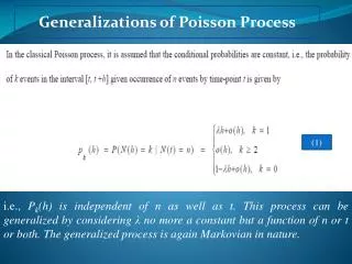
Natural assumption without information • Without further information we have to make the simplest and most natural assumption: • The nobjects occur at independent and uniformly distributedtiming in an interval (0, t), which are then represented by n uniform i.i.d. X1, X2, ..., Xn. • The kth smallest value among uniform i.i.d. is called the kthordered statistic, which means the arrival time of the kth object (not Xk in general) and will be denoted by Sk. • The 1st arrival time S1 = min{X1, ... , Xn} is distributed as: • P(S1 > x) = P(Xj> x for all j) = (1x/t)n • This distribution involves both parameters t and n. Prof. Bob Li
Try to simplify the situation This distribution P(S1> x) = (1x/t)ninvolves both parameters t and n. We try to simplify the situation in two different ways: • Let n. Then, S1 simply becomes zero because for all x > 0 • Let t. Then, S1 simply becomes because for all x > 0 Neither way of simplification is interesting. We need a better way. Prof. Bob Li
Exponential distribution Assumption. In t unit times, there are n = t births. Fix the ratio and let both t and n proportionally. The only parameter remaining is . // More precisely, n = t. // Note the unit of per second, per minute, per year, etc. The 1st arrival time S1 is the minimum among t uniform i.i.d. over the interval (0, t). It is distributed according to: = (1x/t)n= = The distribution function and the density function of S1are: F(x) = 1 and f(x) = This is called the exponential distribution with rate . Prof. Bob Li
Poisson distribution The exponential distribution with rate measures the time till one birth. A symmetric consideration is the birth count in one unit time, which is Binomial(t, 1/t) distributed because of n= t births in t unit times. P{exactly k births in t unit times} = = = Let N denote the limit of this birth count as t . Prof. Bob Li
Poisson distribution For all k 0, P(N = k) = = This is called the Poisson distribution with the density . // = limit of Binomial(t, 1/t) distribution as t In conclusion, in the “pure birth model” with parameter : • Time till one birth is Exponential() distributed. • Birth count in one unit time is Poisson() distributed. Prof. Bob Li
Mean of Poisson Distribution Theorem. Poisson distribution with the density = Poisson distribution with the mean of // per second, per minute,per year, etc. Proof. Let the r.v. N be Poisson() distributed. // Shift the index with k = n1. = // Per second,per minute,per year, etc.
Mean of Exponential Distribution Theorem. Exponential distribution with the rate = Exponential distribution with the mean of 1/ // 1/ seconds, 1/ minutes, 1/ years, etc. Proof. Let M denote an Exponential() r.v. // The letter M hints on the memoryless property of // the exponential distribution given on next page. // Integration by parts = 0 [0 1/] = 1/// 1/ seconds, 1/ minutes, 1/ years, etc.
Memoryless property of exponential distr. Theorem. An exponentially distributed r. v. X is memoryless. More precisely, for all t 0 and x 0, P(X > t+x | X > t) = P(X > x) // Having waited for t unit times, the residual waiting time // still has the same distribution. Or, 不要問我來咗幾耐 Proof. P(X> t+x | X > t) = P(X> t+x) / P(X > t) // x 0 = // Exponential() distribution = = // A memoryless distribution is nonnegative. Prof. Bob Li
Discrete memoryless distribution • The discrete analogue is the geometric distribution. • Geometric0(p) distribution satisfies: • P(N t+x | N t) = P(N x) • Geometric1(p) distribution satisfies: • P(N > t+x | N > t) = P(N > x) Prof. Bob Li
Uniqueness of continuous memoryless distribution Theorem. Exponential distribution is the only continuous memoryless distribution. Proof. Let X be a nonnegative continuous r.v. such that P(X > t+x | X > t) = P(X > x) for all x 0 and t 0. Equivalently, P(X > t+x) = P(X > t)P(X > x) // We need derive an Exponential() distribution function for some . // The natural way to do so is to interpret the property of X as a differential // equation and then solve for a family of functions parameterized by . Differentiating w.r.t. the parameter t, fX(t+x) = fX(t) P(X > x) Setting t = 0, fX(x) = fX(0) P(X > x) …
Uniqueness of continuous memoryless distribution Proof. … fX(x) = fX(0) P(X > x) Writing = fX(0), we arrive at a1st-order differential equation in the variable x P(X > x) fX(x) = 0 with the boundary condition of P(X > 0) = 1. // Total probability = 1 Thus, 0 = ex[P(X > x) fX(x)] = exP(X > x) = constant = e0P(X > 0) = 11 = 1 P(X > x) = e−x// For all x 0 Prof. Bob Li
Waiting for Godot Homework. You are waiting for Godot, who will arrive on the Nth bus, where N is Geometric1(p) distributed. The interarrival times of buses are exponential i.i.d with the intensity . What is the distribution of your waiting time for Godot? Hint: Combine memoryless properties and uniqueness of exponential and geometric distributions. Prof. Bob Li
Transform A transform means an alternative expression for a mathematical object. Example. For an electric wave f(t), where t = time, the Fourier transform () = e-it f(t) dt is an alternative way to specify the function: Given the value () for all , the function f(t) is uniquely determined. The common interpretation of the variable is the frequency, and the value () specifies the amplitude at the particular frequency . In short, the one-to-one correspondence f(t)|a<t<b()|0<< is a transform between the time domain and the frequency domain. Prof. Bob Li
Transforms of an r.v. (or a distribution) The transform of a continuous r.v. X means the transform of its distribution function FX(t) = P(X < t). Definition. When X 0, the Laplace transform of X is () = E[eX], 0. Fact. When X() is known for all , the distribution of X is completely determined. // Qualification of a transform Theorem 1. Let Mbe an Exponential() r.v. and X be an independent r.v. Then, X() = P(X < M) Analogy. The next earthquake will occur at an exponential random time at the rate . A person with the residual lifespan X will miss the next earthquake with the probability P(X < M) = X(). Prof. Bob Li
Transforms of an r.v. (or a distribution) Definition. When X 0, the Laplace transform of X is () = E[eX], 0. Theorem 1. Let Mbe an Exponential() r.v. and X be an independent r.v. Then, X() = P(X < M). Proof. // dFX(x) = fX(x) dx // M is independent of X = E[eX] Prof. Bob Li
Laplacetransform of expon. distribution Theorem 2. TheLaplace transform of an Exponential() r.v. X is X() = / (+) Computational Proof. // FX(x) = 1 ex = / (+) Prof. Bob Li
Laplacetransform of expon. distribution Theorem. TheLaplace transform of an Exponential() r.v. X is X() = / (+) Alternative proof by the pure birth model. Arrival times of telephone calls at the switching center form uniform i.i.d. over the interval [0, t]. There are t tolled telephone calls and t toll-free calls. When t, let the r.v. X represent the arrival time of the first tolled call and the independent r.v. M the arrival time of the first toll-free call. From Theorem 1, TheLaplace transform of X = P(X < M) = limt P(1st tolled call arrives before 1st toll-free call ) = limt P(overall first call is a tolled call) = / (+) // Equal chance for all i.i.d. to win the race 人海战术 Prof. Bob Li
Fourier transform Definition. The Fourier transform of a continuous r.v. X is () = E[e-iX]. Example.For the exponential() r.v., the Fourier transform is () = / (+i), as an analog to the Laplace transform /(+). From this, one can calculate for the exponential distribution as follows: Prof. Bob Li
z-transform Definition. The z-transform of a discrete r.v. X ≥ 0 is = E[zX] = P{Getting all heads in X tosses on a z-biased coin} // z = P{head} = P{X < Mz}, where Mz is an indep. Geometric1(1z) r.v. // 1z = P{tail} // Mz represents the number of coin tosses until the first tail. = P{X ≤ M’z}, where M’zis an indep. Geometric0(1z) r.v. // M’zrepresents the number of coin tosses before the first tail. = The discrete analogue of the Laplace transform Example. The z-transform for a Poisson() r.v. is Prof. Bob Li
Interpretation(To be further clarified after the discussion on splitting aPoisson process) • Telephone calls arrive at the switching center at the rate . Over the interval [0, t], there are t calls. • For each call, we toss a z-biased coin: Head for a tolled call and Tail for a toll-free call. Over the interval [0, t], there are t(1z)toll-free calls. • As t, let a Poisson((1z)) r.v. Xtfrepresent the total number of toll-free arrivals in the interval [0, 1]. Thus, • e(1z) • = P(Xtf= 0) • = P(0 toll-free calls in the interval[0, 1]) • = P{All Poisson() tosses of a z-biased coin show heads} • = The z-transform for a Poisson() r.v. • Homework. Find the z-transform for a Geometric1() r.v. with or without calculation. Prof. Bob Li
Lecture 6 Feb. 27, 2013 Prof. Bob Li
4.2 Combining & splitting of Poisson random variables Prof. Bob Li
Sum of independent Poisson is Poisson. Theorem. Let X and Y be independent Poisson r.v. with respective densities and . Then X+Y is Poisson(+). Computational Proof. P(X+Y = n) = = // Indep. events for fixed k & n = = = = Prof. Bob Li
Alternative proof by z-transform The z-transform for a Poisson() r.v. is E[zX] = . Similarly, E[zY] = . Thus, E[zX+Y] // z-transform for X+Y = E[zXzY] = E[zX] E[zY] // Independence between X and Y = // From previous calculation = = z-transform for a Poisson(+) r.v. Prof. Bob Li
S T t Intuitive proof by pure birth model Consider (+)t uniform i.i.d. over the interval [0, t] representing arrivals ofphone calls at a telephone exchange, where t of them are toll-free calls and t are tolled. As t, the pure birth model leads to the following: • The number of toll-free calls during [0, 1] is Poisson(). • The number of tolled calls during [0, 1] is Poisson(). • These two Poisson random variables are independent, since toll-free calls are independent of tolled calls. • The total number of calls during [0, 1] is Poisson with the mean +.
Minimum of indep. exponential is exponential. Dual Theorem. Let S and T be independent exponential r.v. with respective rates and . Then, min{S, T} is Exponential(+) distributed. Proof. Think of S, T, and min{S, T}, respectively, as the arrival times for the 1st toll-free call, 1st tolled call, and 1st call overall. Then, apply the theorem of “Sum of independent Poisson is Poisson.” Prof. Bob Li
Repairman of machines • Example. There are m machines and a single repairman in a shop. Assume that: • The rate for each machine to break down is per nanosecond, that is, the running time of a machine until breaking down is geometrically distributed, which is approximately Exponential() nanoseconds. • The repairman works on only one broken machine at a time, and the rate of repairing is per nanosecond, that is, the amount of repair time is Exponential() nanoseconds. • The events of breaking down or getting repaired for all machines are independent. • What is the distribution and the average number of downed machines in the long run? Prof. Bob Li
Repairman of machines (cont’d) Construct a markov chain with the state space is {0, 1, …, m}, where the state n is the number of machines that are down. The following diagram shows the transition rates rn,n+1= (mn) and rn,n1 = . // An arrow = a state change. The transition rate means the // transition probability when the unit time = nanosecond. Let (P0P1 … Pm)be the stationary state of the markov chain. Since the states form a string in the transition diagram, the markov chain is time-reversible. Thus, we have balanced flow between every two adjacent states. // “Balanced flow” between every two states gives the same result as // “eigenvector of transition matrix” but simplifies the difference equation. Prof. Bob Li
Repairman of machines (cont’d) [m(n1)]Pn1 = Pn Pn = [m(n1)]/ Pn1 Through telescoping, Now we invoke the boundary condition. In the long run, the average number of downed machines is
Splitting a Poisson r.v. Lemma. Let X and Y be independent Poisson r.v. with respective densities and . Write p = /(+). Then, under the condition of X+Y = n, the distribution of X is Binomial(n, p). That is, Computational Proof. // Two indep. events for fixed k& n
Proof by the pure birth model Let the arrivals of t toll-free telephone calls and t tolled calls all be uniform i.i.d. over the time interval (0, t). As t, the numbers of toll-free and tolled calls, respectively, over the time interval (0, 1) become independent Poisson with respective densities and . They can therefore be represented by the r.v. X and Y in the Lemma. Given that n of the total (+)t calls fall in the interval (0, 1), the probability for exactly k among these n calls are toll-free is // Like drawing n cards out of a deck of (+)t without replacement Hence P(X = k | X+Y = n) = = = Binomial probability with parameters n and p = /(+)
Splitting a Poisson r.v. • Theorem.A fault of a computer system either is recoverable or leads to a breakdown. Assume the total number of faults is Poisson with density and there is an independent probability p for each fault to become a breakdown. Then: • The number of breakdowns is Poisson(p) distributed. • The number of recoverable faults is Poisson(p) distributed. • These two Poisson r.v. are independent. Prof. Bob Li
Computational proof of (1) Let N represent the total number of faults and X the number of breakdowns. We want to show that X is Poisson(p) distributed. P(X = k) // Conditioning on N // By Lemma // Writing m = n k
Intuitive proof of (1) by the pure birth model Place t faults on the time interval (0, t) according to uniform i.i.d., where t is large. The number of faults in the interval (0, 1) is Binomial(t, 1/t). For any single fault, P{It is a breakdown & falls within the interval (0, 1)} = P(Breakdown)P{Within the interval (0, 1)} // Indep. events = p 1/t = p/t Moreover, this probability is independent for every fault. Thus, the number of breakdowns in the interval (0, 1) is Binomial(t, p/t). Similarly, the number of recoverable faults within (0, 1) is Binomial(t, (1p)/t). As t, the numbers of faults, breakdowns, and recoverables in (0, 1) become Poisson(), Poisson(p), and Poisson((1p)), respectively. // Binomial(t, 1/t) Poisson() when t // Binomial(t, p/t) Poisson(p) when t
Intuition behind (3) by the pure birth model The aforementioned distributions Binomial(t, p/t) and Binomial(t, (1p)/t) are negatively correlated to each other because the four rectangles share the total pool of t. But, as t, the correlation between the two tiny rectangles on the left becomes negligible. // Imagine t snow flurries fall down on a big plain, of // which the area t. The number of flurries gathering // on a roof is essentially independent of other roofs. Prof. Bob Li
Computational proof of (3) Let X represent the number of breakdowns, Y the number of recoverable faults, and N = X+Y. We shall show that X and Y are independent. P(X = k and Y = j) = P(X = k and N = k+j) = P(X = k | N = k+j) P(N = k+j) = P(X = k) P(Y = j) Prof. Bob Li
Method of randomization Conditioning on an r.v. removes the randomness at the cost of having to examine all individual instances. Randomizinga deterministic amount with an r.v. creates randomness. Doing so deliberately is to take advantage of certain independence properties of special distributions. This is illustrated below by a fairy tale and a difficult mathematical problem. Prof. Bob Li
A fairy tale • Decrees in the legendary Random Kingdom stipulate: • The silver coins a person leaves behind must be fairlydistributed to offspring in integer quantities. • The amounts received by all offspring must be independentof each other. • // So as to avoid negative correlations • (3) Every coin can be traded to The King for Poisson(1) many coins. • Example. Four silver coins to three children: • $4 $Sum of 4 independent Poisson(1) r.v. • = $Poisson(4) • = $Sum of 3 independent Poisson(4/3) r.v. Prof. Bob Li
A difficult problem • Put n balls randomly into m large boxes. Calculate the probability that every box gets occupied by at least one ball. // Randomly and independently • Solution. Write • G(n) = P(All m boxes occupied | Total n balls) • // Objective is to calculate G(n) for all n. • N = a Poisson() r.v. • () = P(All m boxes occupied | Total N balls) • Thus () relates to G(n) as follow. • () // Conditioning on N • = (N = n) P(All m boxes are occupied | Total n balls) • = G(n) Prof. Bob Li
A difficult problem • Through the equation • the objective sequence {G(n)}nand // In the discrete index n • the function () // In the continuous variable • uniquely determine each other. This makes one particular type of mathematical transform. // Think of n as the discrete time and as the frequency. • We shall first compute the function () and then transform it into {G(n)}n. • Distribute N many balls randomly into mboxes. Each box independently receives Poisson(/m) balls. Hence • P(Box #1 is occupied | Total N balls) • = P(Box #1 is occupied | Box #1 receives Poisson(/m) balls) • = 1e/m// Independence among boxes Prof. Bob Li
A difficult problem () = P(All m boxes occupied | Total N balls) = (1e/m)m// Independent & identical boxes Next we transform the function () into {G(n)}n. The equation is: Since the right-hand side is in the form of a series expansion with respect to , we shall rewrite the left-hand side into the same form. e(e/m1)m// Binomial expansion of (1 e/m)m // Taylor expansion of e // Interchange order • (1e/m)m Prof. Bob Li
Method of randomization (cont’d) Both sides are series expansion with respect to . Comparison of corresponding coefficients on both sides yields G(n) = // No close-form solution is known though. Prof. Bob Li
4.3 Poisson process Prof. Bob Li
From: R. Cooper, “Introduction to Queueing Theory,” North-Holland, 197x
Five equivalent definitions of Poisson process The Poisson process is a special pure-birth process with ramified characterizations based on its properties in terms of interarrival times, arrival times, and arrival counts. Below we shall offer five most useful definitions for a Poisson process and partially prove the equivalence among them. Exponential interarrival times Limit of ordered statistics Poisson count Independent Poisson increments Conditional ordered statistics
N(t) 4 3 2 1 0 Revisit the pure birth model Write Tk= Sk Sk1 = the interarrival time in the pure birth model. // S0 = 0 T1 T2 T3 T4 t S4 0 S2 S3 S1 • The pure birth model can be described in three ways: • Theinterarrival times T1, T2, T3, … // Discrete index, continuous r.v. Sn= 1jnTjTn= SnSn1 • Thearrival times S0 = 0, S1, S2, S3, … // Discrete index, continuous r.v. N(t) n Sn t • Thearrivalcounts N(t) in [0, t], t 0// Continuousparameter, discrete r.v. t
Definition by pure-birth model The first definition characterizes arrival times of a Poisson process by the “pure birth model” of Section 2.1. Definition-A (Limit of ordered statistics). There are t arrival times represented by uniform i.i.d. over the interval [0, t]. These uniform i.i.d. are sorted into ordered statistics. The arrival time Sn in the Poisson process with the intensity is the nth ordered statistic as t. // Recall that nth ordered statistic = nthsmallest among uniform i.i.d. Prof. Bob Li