Download

1 / 7
80 likes | 162 Vues
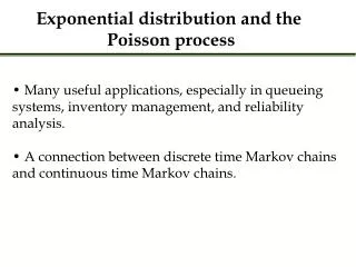
Explore the Poisson distribution, inter-arrival times, and random arrivals in the context of probability theory. From arrival rates to independent random variables, delve into the intricacies and applications of this statistical model.

E N D
CIS 2033 based onDekking et al. A Modern Introduction to Probability and Statistics. 2007 Instructor Longin Jan Latecki C12: The Poisson process
12.2 – Poisson Distribution Definition: A discrete RV X has a Poisson distribution with parameter µ, where µ > 0 if its probability mass function is given by for k = 0,1,2…, where µ is the expected number of rare events occurring in time interval [0, t], which is fixed for X. We can express µ =t λ, where t is the length of the interval, e.g., number of minutes. Hence λ = µ / t= number of events per time unite = probability of success. λ is also called the intensity or frequency of the Poisson process. We denote this distribution: Pois(µ) = Pois(tλ). Expectation E[X] = µ = tλand variance Var(X) = µ = tλ
Let X1, X2, … be arrival times such that the probability of k arrivals in a given time interval [0, t] has a Poisson distribution Pois(tλ): The differences Ti = Xi – Xi-1 are called inter-arrival times or wait times. The inter-arrival times T1=X1, T2=X2 – X1, T3=X3 – X2 … are independent RVs, each with an Exp(λ) distribution. Hence expected inter-arrival time is E(Ti) =1/λ. Since for Poisson λ = µ / t= (number of events) / (time unite) = probability of success, we have for the exponential distribution E(Ti) =1/λ = t / µ = (time unite) / (number of events) = wait time
Let X1, X2, … be arrival times such that the probability of k arrivals in a given time interval [0, t] has a Poisson distribution Pois(λt): Each arrival time Xi, is a random variable with Gam(i, λ) distribution for α=i : We also observe that Gam(1, λ) = Exp(λ):
12.2 –Random arrivals • Example: Telephone calls arrival times • Calls arrive at random times, X1, X2, X3… • Homegeneity aka weak stationarity: is the rate lambda at which arrivals occur in constant over time: in a subinterval of length u the expectation of the number of telephone calls is λu. • Independence: The number of arrivals in disjoint time intervals are independent random variables. • N(I) = total number of calls in an interval I • Nt=N([0,t]) • E[Nt] = t λ • Divide Interval [0,t] into n intervals, each of size t/n
12.2 –Random arrivals • When n is large enough, every interval Ij,n = ((j-1)t/n , jt/n] contains either 0 or 1 arrivals.Arrival: For such a large n ( n > λ t), Rj = number of arrivals in the time interval Ij,n, Rj = 0 or 1 • Rj has a Ber(p) distribution for some p.Recall: (For a Bernoulli random variable)E[Rj] = 0 • (1 – p) + 1 • p = p • By Homogeneity assumption for each jp = λ• length of Ij,n = λ (t / n) • Total number of calls:Nt = R1 + R2 + … + Rn. • By Independence assumption Rj are independent random variables, so Nt has a Bin(n,p) distribution, with p = λ t/n • When n goes to infinity, Bin(n,p) converges to a Poisson distribution