Poisson Random Process
Poisson Random Process. Mean and Variance Results. Exponential:. You have to memorize these! You should be able to derive any of the above. Poisson:. Geometric:. Binomial:. CMPE 252A: Computer Networks SET 3:. Medium Access Control Protocols. APPLICATION. logical link control.
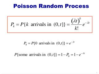

Poisson Random Process
E N D
Presentation Transcript
Mean and Variance Results Exponential: You have to memorize these! You should be able to derive any of the above Poisson: Geometric: Binomial:
CMPE 252A: Computer NetworksSET 3: Medium Access Control Protocols
APPLICATION logical link control Sharing of link and transport of data over the link PRESENTATION SESSION medium access control TRANSPORT NETWORK LINK PHYSICAL Medium Access Control Protocols • Used to share the use of transmission media that can be accessed concurrently by multiple users.
Contention-Based MAC Protocols • No coordination: Stations transmit at will when they have data to send (e.g., ALOHA) • Carrier sensing (listen before transmit): Stations sense the channel before transmitting a data packet (e.g., CSMA). • Listen before and during transmission: Stations listen before transmitting and stop if noise is heard while transmitting (CSMA/CD). • Collision avoidance (floor acquisition): Stations carry out a handshake to determine which one can send a data packet (e.g., MACA, FAMA, IEEE802.11, RIMA). • Collision resolution: Stations determine which one should try again after a collision.
ALOHA Protocol • The first protocol for multiple access channels; the first analysis of such protocols (Norm Abramson, Univ. of Hawaii, 1970). • Originally planned for systems with a central base station or a satellite transponder. Two frequency bands; Up link and down link (413MHz, 407MH at 9600bps) Central node retransmits every packet it receives!
ALOHA Protocol • Population is a large number of bursty stations. • Each station transmits a packet whenever it receives it from its user; no coordination with other stations! • Central node retransmits all packets (good or bad) on down link. • Stations decide to retransmit based on the information they hear from central node
no yes transmit Packet ready? delay packet transmission k times compute random backoff integer k wait for a round-trip time positive ack? no yes ALOHA Protocol An integral part of the ALOHA protocol is feedback from the receiver Feedback occurs after a packet is sent No coordination among sources
The ALOHA Channel • We assume: • An (essentially) infinite population of stations. • An ideal perfect down link for the transmission of feedback to senders. • Stations are half duplex; have zero processing delays. • Retransmissions are scheduled such that all packets are statistically independent. • Each packet has the same duration P. • Stations have the same round-trip delay from one other; this time can be much longer than P (irrelevant). • Packet arrivals are Poisson with rate lambda. • Collisions are the only sources of errors.
P user i NEW RET. user j time time time RET. ... sum collision NEW NEW RET. NEW RET. I B I B I B I B I The ALOHA Channel τ NEW • What percentage of time is the channel sending correct packets? This gives us the throughput of the protocol. NEW
is the arrival rate. For convenience, we normalize the arrival rate as: From the definition of throughput: where p is the probability of a successful packet transmission A packet is successful if no packets arrive within P seconds before it starts or while it is being transmitted; accordingly, S 0.18 G 0.5 Throughput of ALOHA Protocol Because arrivals are Poisson and all packets have equal length, every packet has the same probability of being successful. Therefore,
interfering frame node i frame interfering frame time t0 - 1 t0 + 1 t0 Node i’s frame is vulnerable from any arrival in the time interval (t0-1, t0+1] Throughput of ALOHA Protocol packet overlaps with end of packet from node i packet overlaps with start of packet from node i All packets have the same length
packet overlaps with end of packet from node i packet overlaps with start of packet from node i interfering frame node i frame interfering frame time t0 - 1 t0 + 1 t0 Node i’s frame is vulnerable from any arrival in the time interval (t0-1, t0+1] Throughput of ALOHA Protocol Highest throughput when we have one packet for each 2-packet time period
Slotted ALOHA • The throughput of ALOHA can be improved by reducing the time a packet is vulnerable to interference from other packets. • Slotted ALOHA works in a “slotted channel” providing discrete time slots. • Stations can start transmitting only at the beginning of time slots. • The time synchronization needed for slotting is accomplished at the physical layer, and some synchronization is required in many cases anyway.
no Packet ready? yes Wait for start of next slot transmit delay packet transmission k times compute random backoff integer k wait for a round-trip time quantized in slots no yes positive ack? Slotted ALOHA Protocol
i time arrivals Throughput of Slotted ALOHA The vulnerability period of a packet is a slot time: Any arrivals in prior slot collide with packet i If T is the duration of a time slot and G is the normalized packet arrival rate, then We can obtain the same result by computing the likelihood and average length of utilization, idle and busy periods.
P τ user i user j NEW time time time slot NEW NEW RET sum NEW NEW time I B I B B I B Slotted ALOHA RET NEW ... collision IMPORTANT: The starting point of a busy period is a “renewal point”! System is busy
Renewal Theory • Recall the Poisson random process: • N(t) = number of arrivals in (0, t] • Inter-arrival times are exponentially distributed • N(t) is a counting processwith exponential inter-arrival times. • Definition of Renewal Process: A counting process N(t) for which inter-arrival times X1, X2, …, Xn are an independent identically distributed (iid) random sequence.
arrival …. time 1 2 3 k 0 t 1 2 3 4 n Poisson Random Variable A sequence of n independent Bernoulli trials; with X being the number of arrivals in (0, t] By assumption, whether or not an event occurs in a subinterval is independent of the outcomes in other subintervals. We have:
arrival …. time 1 2 3 k 0 1 2 3 4 n Renewal Theory Example • At each time t = 1, 2, …, a Bernoulli process N(t) has an arrival with probability p, and this is independent of the occurrence of arrivals at any other times. • Is N(t) a renewal process?
…. time 0 (1-p) (p) (1-p) Renewal Theory Example • Answer: • For any inter-arrival period n, the inter-arrival time Xn equals x if there were x-1 Bernoulli failures followed by a success. Xn = 3 if we have 2 failures followed by a success! 1 2 3
Renewal Theory Example • Therefore, each inter-arrival time Xn has the Geometric PMF: • Because each Bernoulli trial is independent, Xn is independent of the previous inter-arrival times X1, X2 ,…Xn-1. • This implies that a Bernoulli arrival process is a renewal process!
Renewal Theory • After an arrival (in a renewal process), the subsequent inter-arrival times are distributed identically to the original inter-arrival times. • Effectively, the process restarts, or has a renewal, whenever an arrival occurs!
Renewal Theory • Suppose that N(t) has n arrivals by time t1, the additional time until the next arrival is denoted by Sn+1 - t1, and the subsequent inter-arrival times are Xn+2 , Xn+3 ,… and so on. • Renewal Point:For a renewal process N(t),time t1 with N(t1) = nis a renewal point ifSn+1 - t1, Xn+2, Xn+3,… is an iid random sequence statistically identical to X1, X2, X3,… • Every instant of time is a renewal point for a Poisson process!
time Renewal Theory Alternating renewal process: System is on and off (that is, or busy and idle). system success collision success ... off on off on off on off ... Y1 X1 Y2 X2 Y3 X3 Y4 ... X1, X2, X3,…. are i.i.d. with mean E(X) Y1, Y2, Yx,…, are i.i.d. with mean E(Y) P(t) = P{system is ON at time t in steady state} = E(x)/{E(x)+E(Y)} Average cycle length = E(X) + E(Y)
bad busy period idle period good busy period success failure time Evaluating Throughput • We assume that the system is “stationary,” i.e., system behaves in cycles that are statistically equivalent • Average cycle consists of an idle period (I ) and a busy period (B ). • The busy portion of a cycle has good and part parts. • The portion of time used to send user data is called the utilization period (U )
Evaluating Throughput • The expression for S amounts to simply taking averages. • What we need to do now is compute the probability that I, B (good a bad parts), and U happen in an average cycle, and their average duration. • Ideally, these probabilities are based onindependent events, and we can express S based on knowledge of the present state of the system.
time no arrivals transmissions start arrivals idle period starts Throughput of Slotted ALOHA Idle, busy and utilization periods are multiples of time slots. We need to count the time slots in each average period and we are done. Average length of idle period: I = number of slots in idle period
I has one slot: there is a prior busy period ... ... at least one arrival! time time I has two slots: no arrivals at least one arrival! Idle Period in Slotted ALOHA
I has k slots: 1 k-1 k ... time … some arrivals no arrivals Idle Period in Slotted ALOHA This corresponds to the Geometric r.v., and we know its average value to be 1/p, with p being the probability of success. Success now consists of ending the idle period! Therefore:
… no arrivals B has k slots: ... time 1 k k-1 some arrivals Busy Period in Slotted ALOHA • We follow the same approach: • Solve the problem with the Geometric random variable prior slot considered in idle period
collision sum time Utilization Period • Here we have to make use of conditional probability! • A busy period has good and bad time slots (transmission periods). The probability that a slot (transmission period) in the current busy period is successful is the probability that only one packet arrives in the prior slot, given that there is a busy period Arrivals are Poisson, so we make use of the definition of that random variable as follows….
Utilization Period The probability that a given slot within a busy period is successful is: The portion of an average busy period used to send useful data equals the length of the average busy period in slots, times the probability that any given slot is successful. We can use the Binomial random variable to proof the above!
Throughput of Slotted ALOHA • We now just substitute B,I, and U in S: Maximum throughput is twice that of ALOHA. This occurs when G = 1
Average Delay of MAC Protocols • We want to measure or compute the average time from the instant the first bit of a packet is first transmitted to the moment the last bit is received correctly at the destination. • Assume that arrivals (of new and retransmitted data or control packets) to the channel are Poisson. • Assume fully-connected networks.
The average number of transmissions needed for a packet to be received correctly is Therefore, the number of retransmissions is Average Delay in ALOHA Assumptions: A satellite channel with propagation delay NxP, where P is the packet length and NxP >> P A retransmission is sent after an average backoff time of BxP seconds. Direct method: A packet is transmitted (G/S-1) times in error (due to collisions) and each such transmission wastes P+NxP +BxP seconds. The last transmission is successful and must take P+NxP seconds. Therefore, the average delay incurred is:
START END BACK OFF Average Delay in ALOHA Indirect Method: Based on the fact that the success of a transmission is independent of others, and knowing how many times we have retransmitted does not change the likelihood of success in the next transmission! We use a diagram showing possible states, probabilities of transition, and delay incurred in that transition. From the diagram. we obtain a number of simultaneous equations that we solve to obtain delay from START to END.
From the diagram we have: Substituting we obtain the same result expected from the Geometric r.v. Average Delay in ALOHA Solving these two equations: The same method can be applied on the other MAC protocols!
Average Delay of ALOHA • The delay increases exponentially with heavy load, which is not acceptable for real-time applications.
CSMA: Carrier Sense Multiple Access • The capacity of ALOHA or slotted ALOHAis limited by the large vulnerability period of a packet. • By listening before transmitting, stations try to reduce the vulnerability period to one propagation delay. • This is the basis of CSMA (Kleinrock and Tobagi, UCLA, 1975) • Many of the assumptions made for ALOHA are made now for CSMA.
Channel Busy? Packet ready yes no transmit delay packet transmission k times wait for a round-trip time positive ack? compute random backoff integer k no yes CSMA Protocol Assume non-persistent carrier sensing. Requires a maximum propagation delay much smaller than packet lengths!
CSMA Throughput A virtualsecondary channel used to send ACKs reliable and in 0 time! Same assumptions made for pure ALOHA analysis. All stations are at one propagation delay from each other and that equals: Arrivals are Poisson with average rate Peer-to-peer communication No base station or transponder Explicit feedback to sender!
P user i RET NEW user j time time time NEW RET. ... sum collision NEW RET NEW RET. I B I B I B I CSMA Protocol τ The big difference compared to ALOHA is that busy periods are bounded!
P time successful period failed period collision NEW RET. NEW RET. I B I B I B I CSMA Throughput We can approximate: Length of average idle period (exponential interarrivals)? The probability that a packet is successful is? (no packets can arrive within tau sec. after the start of the packet!) The average length of a utilization period is?
START END P LAST FIRST time Y Y Y is a random variable! CSMA Throughput Pretty accurate for << P Substituting we have: More accurate estimation of S requires finding the average length of B.
START Y =y LAST FIRST time no arrivals, no more arrivals occur after LAST CSMA Throughput Note that the average length of B is determined by the time between the start of the first and the last packet in the busy period.
CSMA Throughput Substituting we get: Approximate:
Channel Busy? Packet ready yes no wait for start of next slot transmit delay packet transmission k times wait for a round-trip time quantized in slots positive ack? compute random backoff integer k no yes Slotted CSMA • Non-persistent strategy. • A slot lasts one maximum propagation delay.
I has k slots: collision success 1 k-1 k ... time RET. NEW … some arrivals time no arrivals P I B I B I Just as in slotted ALOHA, with slot duration equal to Computing the Throughput of Slotted CSMA
Slotted CSMA: ... time k-1 1 k … no arrivals in last slot of last transmission period some arrivals in last slot of each transmission period Throughput of Slotted CSMA • We follow the same approach as in slotted ALOHA • B has k transmission periods, each of P + τ sec • What happens in a transmission period depends only on the last time slot of the prior transmission period!