Download
1 / 40
400 likes | 609 Vues
Background Error Covariance Modeling. Craig H. Bishop Naval Research Laboratory, Monterey (with many slides taken from Mike Fisher’s ECMWF lecture on the same subject) JCSDA Summer Colloquium July 2012 Santa Fe, NM. Overview. Covariances of what, precisely?

E N D
Background Error Covariance Modeling Craig H. Bishop Naval Research Laboratory, Monterey (with many slides taken from Mike Fisher’s ECMWF lecture on the same subject) JCSDA Summer Colloquium July 2012 Santa Fe, NM
Overview • Covariances of what, precisely? • Static error covariances from observations • Error covariances from proxies • Bayes’ theorem • Perturbed observation ensembles • Kalman filters and EnKF ensembles • Computationally efficient static error covariances. • Inclusion of balance constraints • Conclusions
What is the true error distribution ? (Slartibartfast – Magrathean designer of planets, D. Adams, Hitchhikers …) • Imagine an unimaginably large number of quasi-identical Earths.
Why do error covariances matter? • The temperature forecast for Albuquerque is much colder than the verifying observation by 5K. Does this mean that the forecast for Santa Fe was also to cold? • What if the forecast error was associated with an approaching cold front? • How would the orientation of the cold front change your answer to question 1?
Problem • We don’t know the true state and hence cannot produce error samples. • We can attempt to • infer forecast error covariances from innovations (y-Hxf) (e.g. Hollingsworth and Lohnberg, 1986, Tellus) • And/or • create proxies of error from first principals (e.g. ensemble perturbations)
Static forecast error covariances from innovations An attractive property of the HL method is that its estimates are entirely independent of the estimates of P and R that are used in the data assimilation scheme. Hollingsworth-Lönnberg Method (Hollingsworth and Lönnberg, 1986) Ob error variance Rii Includes uncorrelated error of representation Extrapolate green curve to zero separation, and compare with innovation variance Fcst error variance Pii Desrozier’s method depends on differences between analyses and observations. These differences are entirely dependent on the assumptions made in the DA scheme. Innovation covariances binned by separation distance Desroziers’ Method (Desrozierset al 2005) From O-F, O-A, and A-F statistics, the observation error covariance matrix R, the representer HBHT, and their sum can be diagnosed
Static forecast error covariances from innovations Bauer et al., 2006, QJRMS
Why does the correlation function for the AIREP data look qualitatively different to that from the SSMI radiances? C/O Mike Fisher
Pros and cons of error covariances from binned innovations • Pros • Ultimately, observations are our only means to perceive forecast error. • Innovation based approaches enable both forecast error covariances and observation error variances to be simultaneously estimated. • Cons • Only gives error estimates where there are observations (what about the deep ocean, upper atmosphere, cloud species, etc) • Provides extremely limited information about multi-variate balance. • Limited flow dependent error covariance information.
Covariances of proxies of forecast error • Parish and Derber’s (1992, MWR)“very crude 1st step” using the difference between a 48 hr and 24 hrfcsts valid at the same time as a proxy for 6 hrfcst error has been widely used. • Oke et al. (2008, Ocean Modelling) use deviations of state about 3 month running average as a proxy for forecast error. • Both 1 and 2 can be made to be somewhat consistent with innovations How could we produce better proxies of forecast error?
Covariances of proxies of forecast error • Forecast error distributions depend on analysis error distributions and model error distributions. • Analysis error distributions depend on the data assimilation scheme used and the location and accuracy of the observations assimilated. • Estimation of these distributions is difficult in practice but there is theory for it.
Prior pdf of truth Probability density Ensemble forecasts are used to estimate this distribution. They are a collection of weather forecasts started from differing but equally plausible initial conditions and propagated forward using a collection of equally plausible dynamical or stochastic-dynamical models. Value of truth
Likelihood density function In interpreting the likelihood function (red curve) note that y is fixed at y=1. The red curve describes how the probability density of obtaining an error prone observation of y=1 varies with the true value xt. Value of truth
Posterior pdf Probability density No operational or near operational data assimilation schemes are capable of accurately representing such multi-modal posterior distributions. Value of truth
Ensemble of perturbed obs 4DVARS does not solveBayes’ theorem Green line is pdf of ensemble of converged perturbed obs 4DVARs having the correct prior and correct observation error variance. Blue line is the pdf of ensemble of 4DVARS after 1st inner loop (not converged) Black line is the true posterior pdf.
EnKF doesn’t solveBayes’ theorem either Cyan line is posterior pdf from EnKF Black line is the true posterior pdf.
Recapitulation on proxy error distributions • Ensembles of 4DVARs and/or EnKFs provide accurate flow dependent analysis and forecast error distributions provided all error distributions are Gaussian and accurately specified. • In the presence of non-linearities and non-Gaussianity, the 4DVAR/EnKF proxies are inaccurate but probably not as inaccurate as proxies for which 1 does not hold. • One can use an archive of past flow dependent error proxies to define a static or quasi-climatological error covariance. (Examples follow)
Computationally Efficient Quasi-Static Error Covariance Models
Boer, G. J., 1983: Homogeneous and Isotropic Turbulence on the Sphere. J. Atmos. Sci., 40, 154–163. Pointed out that isotropic correlation functions on the sphere are obtained from EDE^T where E is a matrix listing spherical harmonics and D is a diagonal matrix whose values (variances) only depend on the total wave number.
Wavelet transforms permit a compromise between these two extremes. ECMWF currently has a wavelet transform based background error covariance model. May have time to touch on this tomorrow.
Divergence without omega equation Divergence with omega equation
Sophisticated balance operators impart a degree of flow dependence to both the error correlations and the error variances!
Recapitulation on today’s lecture • Differences between forecasts and observations can be used to infer aspects of spatio-temporal averages of • Observation error variance • Forecast error variance • Quasi-isotropic error correlations • Monte Carlo approaches (Perturbed obs 3D/4D VAR, EnKF) and deterministic EnKFs(ETKF, EAKF, MLEF) provide compelling error proxies for both flow-dependent error covariance models and flow-dependent error covariance models. • In variational schemes, the need for cost-efficient matrix multiplies has led to elegant idealizations of the forecast error covariance matrix • sophisticated balance constraints can be built into these models. • There were many approaches I did not cover (Recursive filters, Wavelet Transforms, etc). • Tomorrow: Ensemble based flow dependent error covariance models