Background Error Covariance Modeling
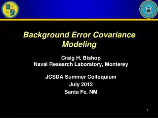
Background Error Covariance Modeling. Craig H. Bishop Naval Research Laboratory, Monterey JCSDA Summer Colloquium July 2012 Santa Fe, NM. Overview. Strategies for flow dependent error covariance modeling Ensemble covariances and the need for localization

Background Error Covariance Modeling
E N D
Presentation Transcript
Background Error Covariance Modeling Craig H. Bishop Naval Research Laboratory, Monterey JCSDA Summer Colloquium July 2012 Santa Fe, NM
Overview • Strategies for flow dependent error covariance modeling • Ensemble covariances and the need for localization • Non-adaptive ensemble covariance localization • Adaptive ensemble covariance localization • Scale dependent adaptive localization • Flexibility of localization scheme allowed by DA algorithm. • Hidden error covariances and the need for a linear combination of static-climatological error covariances and flow dependent covariances. • New theory for deriving weights for Hybrid covariance model from (innovation, ensemble-variance) pairs • Conclusions
Small Ensembles and Spurious Correlations Stable flow error correlations km Unstable flow error correlations km Ensembles give flow dependent, but noisy correlations
Small Ensembles and Spurious Correlations Stable flow error correlations Fixed localization Most ensemble DA techniques reduce noise by multiplying ensemble correlation function by fixed localization function (green line). Resulting correlations (blue line) are too thin when true correlation is broad and too noisy when true correlation is thin. km Unstable flow error correlations Fixed localization km Fixed localization functions limit adaptivity
Small Ensembles and Spurious Correlations Stable flow error correlations t = 0 • Current ensemble localization functions poorly represent propagatingerror correlations. km Unstable flow error correlations t = 0 km Fixed localization functions limit ensemble-based 4D DA
Small Ensembles and Spurious Correlations Stable flow error correlations t = 0 t = 1 • Current ensemble localization functions poorly represent propagatingerror correlations. km Unstable flow error correlations t = 0 t = 1 km Fixed localization functions limit ensemble-based 4D DA
Small Ensembles and Spurious Correlations Stable flow error correlations t = 0 t = 1 • Green line now gives an example of one of the adaptive localization functions that are the subject of this talk. km Unstable flow error correlations t = 0 t = 1 km Want localization to adapt to width and propagation of true correlation
Bayesian perspective onlocalization Ideally, localization would yield the mean or mode of the posterior based on informed guesses of the prior and likelihood distributions.
Prior correlation distribution might be a function of: • distance from sample correlation of 1 • latitude, longitude, height • Rossby radius, Richardson number • estimated geostrophic coupling (for multi-variate case) • estimated group velocity of errors (for variables separated in time) • anisotropy of nearby features (e.g. fronts) Non-adaptive localization Adaptive localization How about trying to extract this info from the ensemble?
1 128 256 1 128 256 (b) (a) (c) (d) Smoothed ENsembleCOrrelationsRaised to a Power (SENCORP)(Bishop and Hodyss, 2007, QJRMS) Bishop and Hodyss, 2007, QJRMS. In matrix form,
Ensemble COrrelations Raised to A Power (ECO-RAP) Bishop and Hodyss, 2009ab, Tellus (a) (b) K = 64 member ensemble Ensemble correlation matrix nelementwise products of ensemble correlation (c) (d) Non-adaptive localization matrix
Bishop and Hodyss, 2009ab, Tellus • Nice features of ECO-RAP include: • Reduces to a propagating non-adaptive localization in limit of high power • Can apply square root theorem and separability assumption to reduce memory requirements
Square root theorem provides memory efficient representation (Bishop and Hodyss, 2009b, Tellus) Modulated ensemble Modulated ensemble member Root is huge ensemble of modulated ensemble members! K2(K+1)/2can be linearly independent (K=128 => a possible 1,056,768 linear independent members)
Example of a modulated ensemble member Raw ensemble member k Smooth ensemble member j Modulated ensemble member Smooth ensemble member i
Data Assimilation using Modulated EnsembleS (DAMES) using Navy global atmospheric model, NOGAPS
18 Z 12 Z (a) (b) Sigma Level Sigma Level (d) (c) Longitude Longitude No localization Unlocalized ensemble covariance function of meridional wind at 18 UTC and 12 UTC with 18 UTC meridional wind variable at 90E, 40S sigma-level 15 (about 400 hPa). Bishop, C.H. and D. Hodyss, 2011: Adaptive ensemble covariance localization in ensemble 4D-VAR state estimation, Mon. Wea . Rev.139, 1241-1255.
18 Z 12 Z (a) (b) Sigma Level Sigma Level (c) (d) Longitude Longitude Adaptive localization Ensemble covariance function localized with the partially adaptive ensemble covariance localization function (PAECL). Bishop, C.H. and D. Hodyss, 2011: Adaptive ensemble covariance localization in ensemble 4D-VAR state estimation, Mon. Wea . Rev.139, 1241-1255.
18 Z 12 Z (a) (b) Sigma Level Sigma Level (c) (d) Longitude Longitude Non-adaptive localization Ensemble covariance function localized with the non-adaptive ensemble covariance localization (NECL).
(a) (b) Sigma Level Sigma Level (c) (d) Longitude Longitude Thisstudy was only able to compare the performance of the two schemes over a long enough period to establish any significance between the performance of non-adaptive and adaptive localization. In simpler models, adaptive localization has been shown to beat or match the performance of non-adaptive localization – depending on the need for adaptive localization. Comparison of structure of optimally tuned adaptive (a) and non-adaptive (b) localization functions at 12 UTC. Fig’s (c) and (d) give the corresponding vertical structure of the adaptive and non-adaptive localization functions along the N latitude circle.
Synoptic scales need to be analyzed 1,000 km
so do mesoscales, 100 km 100 km
Motivation: Our Multi-Scale World Convection near a mid-latitude cyclone Simple Model Ensemble Perturbation
Motivation: Our Multi-Scale World Convection near a mid-latitude cyclone Red – True 1-point covariance Black – 32 member ensemble 1-point covariance
Will traditional localization help? Localization with Broad Function Localization with Narrow Function Green – Localized 1-point covariance
Now imagine the convection is moving … Initial Time Final Time Red – True 1-point covariance Black – 32 member ensemble 1-point covariance
Will traditional localization help? Localization with Broad Function Initial Time Final Time Green – Localized 1-point covariance
New Method: Multi-scale DAMES • Spatially smooth the ensemble members and call this the large-scale ensemble • Use a step-function in wavenumber space • Subtract the large-scale ensemble from the raw ensemble and call this the small-scale ensemble • This implies a partition like • Apply the DAMES method to expand ensemble size • to each ensemble separately • Create localization ensemble members, i.e. choose variable and smooth • Use modulation products to construct “modulation” ensemble members • Add modulation ensemble members from the large-scale ensemble and the small-scale ensemble together to form one set of modulation ensemble members • This implies that the final ensemble looks like
Decompose into large and small-scale portions … Large-Scale Ensemble Perturbation Small-Scale Ensemble Perturbation
DAMES: Step 1 – Smooth the perturbations Smoothed Large-Scale Ensemble Perturbations (Smooth Member 1) (Smooth Member 2)
DAMES: Step 2 – Modulate smooth members and normalize the resulting ensemble Large-Scale Ensemble Perturbations (Smooth Member 1) x (Smooth Member 2) Associated Localization Function
DAMES: Step 3 – Modulate raw member Large-Scale Ensemble Perturbations (Raw Member 2) x (Smooth Member 1) x (Smooth Member 2) This is a modulation ensemble member!
Large-Scale and Small-Scale Perturbations (Raw Member 2) x (Smooth Member 1) x (Smooth Member 2) Small-Scale Ensemble Perturbation Large-Scale Ensemble Perturbation
The MS-DAMES Ensemble Recall that the MS-DAMES modulation ensemble is the sum of the large-scale and small-scale members: Subsequent research has shown that treating the small and large scale modulated members as individual members (rather than adding them together) actually works better.
1-point Covariance functions The Multi-scale DAMES algorithm gave a qualitatively good result! Initial Time Final Time Red – True 1-point covariance Green – Non-adaptively localized covariance Blue – Multi-scale DAMES covariance
Have we localized the covariance? Effective Localization Blue – MS-DAMES 1-point covariance Black – Raw 1-point covariance
Let’s Assimilate Some Obs … The MS-DAMES algorithm gave a superior quantitative result • Two cases: Observe every point at the final time with ob error = 0 or 1 • Obtain the initial state using the modulation ensemble to propagate the effect of the obs back in time • 16 trials: • Initial time RMS(Analysis Error) • Ob error = 0 Ob error = 1 • Optimal 0.27 0.61 • MS-D 0.31 0.63 • Non-adapt 1.4 0.92 Initial Time Analysis Error (R = 0) Red – Optimal Green – Non-adaptive Blue – MS-DAMES
Summary • Ensemble based error covariance models require some form of covariance localization that serves to (a) increase the effective ensemble size, and (b) attenuate spurious correlations. • When errors (a) move a significant distance relative to their correlation length scale over the DA window and/or (b) exhibit differing scales at differing locations, adaptive localization can significantly improve the covariance model. • When differing error scales move in differing directions multi-scale ensemble covariance localization is likely to be of use.
Current DA ill-suited to multi-scale problem Multiscale correlation functions. In (a) and (b) red lines give the true covariance of variables in 256 variable model at t=0 and t=12, respectively, with the 128th variable at t=0. Blue lines give the corresponding raw ensemble covariance from a 32 member ensemble. Black lines give the corresponding localized ensemble covariance. Green lines give the non-adaptive localization function used to localize the ensemble covariances. Current physical space ensemble covariance localization techniques inadequate for multi-scale problem
Naval Research Laboratory Marine Meteorology Division Monterey, California Adaptive Localization needed because: • True error correlation length scale is a function of time and location • The location of correlated errors propagates through time • Multiple error correlation length scales may exist simultaneously
What is the true error distribution ? (Slartibartfast – Magrathean designer of planets, D. Adams, Hitchhikers …) • Imagine an unimaginably large number of quasi-identical Earths.
Why do error covariances matter? • The temperature forecast for Albuquerque is much colder than the verifying observation by 5K. Does this mean that the forecast for Santa Fe was also to cold? • What if the forecast error was associated with an approaching cold front? • How would the orientation of the cold front change your answer to question 1?
Problem • We don’t know the true state and hence cannot produce error samples. • We can attempt to • infer forecast error covariances from innovations (y-Hxf) (e.g. Hollingsworth and Lohnberg, 1986, Tellus) • And/or • create proxies of error from first principals (e.g. ensemble perturbations)
Static forecast error covariances from innovations An attractive property of the HL method is that its estimates are entirely independent of the estimates of P and R that are used in the data assimilation scheme. Hollingsworth-Lönnberg Method (Hollingsworth and Lönnberg, 1986) Ob error variance Rii Includes uncorrelated error of representation Extrapolate green curve to zero separation, and compare with innovation variance Fcst error variance Pii Desrozier’s method depends on differences between analyses and observations. These differences are entirely dependent on the assumptions made in the DA scheme. Innovation covariances binned by separation distance Desroziers’ Method (Desrozierset al 2005) From O-F, O-A, and A-F statistics, the observation error covariance matrix R, the representer HBHT, and their sum can be diagnosed
Static forecast error covariances from innovations Bauer et al., 2006, QJRMS