Parsimony method
Parsimony method. Jarno Tuimala Thanks to James McInerney for the slides with a darker background!. Topics. Theory of parsimony method Evolutionary models (optimality criterion) in parsimony Finding optimal trees Consensus trees Checking reliability. Ideas behind parsimony.

Parsimony method
E N D
Presentation Transcript
Parsimony method Jarno Tuimala Thanks to James McInerney for the slides with a darker background!
Topics • Theory of parsimony method • Evolutionary models (optimality criterion) in parsimony • Finding optimal trees • Consensus trees • Checking reliability
Development of parsimony method • Willi Hennig 1950 • ”Assumes that the tree that gives the fewest number of character state changes along the branches of a tree gives the best estimate of phylogeny of the characters being examined” (Fitch 2003) • Farris 1969 • Parsimony on ordered characters (morphology) • ”Wagner trees” • Fitch 1970-1971 • Parsimony on unordered characters (nucleotides) • Sankoff 1973 • Generalized parsimony • Felsenstein 1978 • Introduces maximum likelihood to phylogenetics, and shows that parsimony could be inconsistent (”Felsenstein zone”)
Characters • Organisms are a set of features (characters): 0123456789AB ACGTAGCTGAGT ACGTAGCTGAGT CCGTAGCAGAGT CCGTAGCAGAGT CCGTAGCAGAGT • When organisms differ with respect to a feature, different feature forms are called character states
Unique and unreversed characters (apomorphy) • Because hair evolved only once and is unreversed (not subsequently lost) it is homologous and provides unambiguous evidence of relationships Human Lizard HAIR absent present Dog Frog change or step
Homoplasy - misleading evidence of phylogeny • If misinterpreted as homology, the absence of tails would be evidence for a wrong tree: grouping humans with frogs and lizards with dogs Lizard Human TAIL absent present Dog Frog
Homoplasy - independent evolution • Loss of tails evolved independently in humans and frogs - there are two steps on the true tree Human Lizard TAIL (adult) absent present Dog Frog
Homoplasy - reversal • Reversals are evolutionary changes back to an ancestral condition • As with any homoplasy, reversals can provide misleading evidence of relationships True tree Wrong tree 9 1 3 4 6 7 7 8 3 4 6 2 5 8 9 10 1 2 5 10
Homoplasy in molecular data • Incongruence and therefore homoplasy can be common in molecular sequence data • There are a limited number of alternative character states ( e.g. Only A, G, C and T in DNA) • Rates of evolution are sometimes high • Character states are chemically identical • homology and homoplasy are equally similar • cannot be distinguished by detailed study of similarity and differences
Incongruence or Incompatibility Human Lizard • These trees and characters are incongruent - both trees cannot be correct, at least one is wrong and at least one character must be homoplastic HAIR absent present Dog Frog Lizard Human TAIL absent present Dog Frog
Congruence • We prefer the ‘true’ tree because it is supported by multiple congruent characters Human Lizard MAMMALIA Hair Single bone in lower jaw Lactation etc. Dog Frog
Parsimony analysis • Parsimony methods provide one way of choosing among alternative phylogenetic hypotheses • The parsimony criterion favours hypotheses that maximise congruence and minimise homoplasy • It depends on the idea of the fit of a character to a tree
Character Fit • Initially, we can define the fit of a character to a tree as the minimum number of steps required to explain the observed distribution of character states among taxa • This is determined by parsimonious character optimization • Characters differ in their fit to different trees
Parsimony Analysis • Given a set of characters, such as aligned sequences, parsimony analysis works by determining the fit (number of steps) of each character on a given tree • The sum over all characters is called Tree Length • Most parsimonious trees (MPTs) have the minimum tree length needed to explain the observed distributions of all the characters
Parsimony in practice Of these two trees, Tree 1 has the shortest length and is the most parsimonious Both trees require some homoplasy (extra steps)
Results of parsimony analysis • One or more most parsimonious trees • Hypotheses of character evolution associated with each tree (where and how changes have occurred) • Branch lengths (amounts of change associated with branches) • Various tree and character statistics describing the fit between tree and data • Suboptimal trees - optional
Character types • Characters may differ in the costs (contribution to tree length) made by different kinds of changes • Wagner (ordered, additive) • 012(morphology, unequal costs) • Fitch(unordered, non-additive) • A G (morphology, molecules) • TC (equal costs for all changes) one step two steps
Character types • Sankoff (generalised) • A G (morphology, molecules) • TC (user specified costs) • For example, differential weighting of transitions and transversions • Costs are specified in a stepmatrix • Costs are usually symmetric but can be asymmetric also (e.g. costs more to gain than to loose a restriction site) one step five steps
To ACGT A 0 515 C5 0 51 From G15 0 5 T515 0 Stepmatrices • Stepmatrices specify the costs of changes within a character PURINES (Pu) A G transversions Py Pu T C PYRIMIDINES (Py) transitions Different characters (e.g 1st, 2nd and 3rd) codon positions can also have different weights Py Py Pu Pu
Different kinds of changes differ in their frequencies To A C G T Transitions A Transversions C From Unambiguous changes on most parsimonious tree of Ciliate SSUrDNA G T
Weighted parsimony • If all kinds of steps of all characters have equal weight then parsimony: • Minimises homoplasy (extra steps) • Maximises the amount of similarity due to common ancestry • Minimises tree length • If steps are weighted unequally parsimony minimises tree length - a weighted sum of the cost of each character
0 1 2 3 4 5 6 7 8 9 10 11 12 13 14 15 16 17 18 19 20 21 Why weight characters? • Many systematists consider weighting unacceptable, but weighting is unavoidable (unweighted = equal weights) • Transitions may be more common than transversions • Different kinds of transitions and transversions may be more or less common • Rates of change may vary with codon positions • The fit of different characters on trees may indicate differences in their reliabilities • However, equal weighting is the commonest procedure and is the simplest approach 250 200 Ciliate SSUrDNA data 150 Number of Characters 100 50 0 Number of steps
Parsimony can be inconsistent • Felsenstein (1978) developed a simple model phylogeny including four taxa and a mixture of short and long branches • Under this model parsimony will give the wrong tree Long branches are attracted but the similarity is homoplastic • With more data the certainty that parsimony will give the wrong tree increases - so that parsimony is statistically inconsistent • Advocates of parsimony initially responded by claiming that Felsenstein’s result showed only that his model was unrealistic • It is now recognised that the long-branch attraction (in the Felsenstein Zone) is one of the most serious problems in phylogenetic inference
Practical issues • Analysis is usually done using some software package on a computer. • First, an initial tree is created fast, possibly using Wagner method • This initial tree is then rearranged in order to find the shortest (MPT) tree. • Exact solutions • Heuristics!
Development of parsimony method • Hill climbing methods (heuristics) • NNI: Robinson 1971, Moore 1973 • Branch and bound: Hendy, 1982 • SPR: Swofford 1987, 1993 • TBR: Maddison 1991 • Ratchet: Nixon 1999 • TD, TF, SS: Goloboff 1999
Tree space may be populated by local minima and islands of optimal trees RANDOM ADDITION SEQUENCE REPLICATES (RAS or jumble) FAILURE SUCCESS FAILURE Branch Swapping Branch Swapping Tree Branch Swapping Length Local Minimum Local GLOBAL Minima MINIMUM
Finding optimal trees - exact solutions • Exact solutions can only be used for small numbers of taxa • Exhaustive search examines all possible trees • Typically used for problems with less than 10 taxa
Finding optimal trees - exhaustive search B C Starting tree, any 3 taxa 1 A Add fourth taxon (D) in each of three possible positions -> three trees E B D C C D B E B D C 2a 2b 2c E A A A E E Add fifth taxon (E) in each of the five possible positions on each of the three trees -> 15 trees, and so on ....
Finding optimal trees - exact solutions • Branch and bound saves time by discarding families of trees during tree construction that cannot be shorter than the shortest tree found so far • Can be enhanced by specifying an initial upper bound for tree length • Typically used only for problems with less than 18 taxa
Finding optimal trees - branch and bound C2.1 B C C C3.1 D B C A1 C2.2 B C3.2 D C2.3 C3.3 A C2.4 C3.4 B2 B3 A A C2.5 C3.5 B E E B D B D C C D C B1 C1.1 C1.5 A A A B D B D E D E C B C1.3 C C1.2 E C1.4 C A A A
Finding optimal trees - heuristics • The number of possible trees increases exponentially with the number of taxa making exhaustive searches impractical for many data sets (an NP complete problem) • Heuristic methods are used to search tree space for most parsimonious trees by building or selecting an initial tree and swapping branches to search for better ones • The trees found are not guaranteed to be the most parsimonious - they are best guesses
Finding optimal trees - heuristics • Stepwise addition • Asis - the order in the data matrix • Closest -starts with shortest 3-taxon tree adds taxa in order that produces the least increase in tree length (greedy heuristic) • Simple - the first taxon in the matrix is a taken as a reference - taxa are added to it in the order of their decreasing similarity to the reference • Random - taxa are added in a random sequence, many different sequences can be used • Recommend random with as many (e.g. 10-100) addition sequences as practical
Finding most parsimonious trees - heuristics • Branch Swapping: • Nearest neighbor interchange (NNI) • Subtree pruning and regrafting (SPR) • Tree bisection and reconnection (TBR) • Ratchet • Tree fusing • Tree drifting • Sectorial searches
C D E A F B G D C C D E A E A F B F B G G Finding optimal trees - heuristics • Nearest neighbor interchange (NNI)
C D E A F B G E C D F E G C A F B D B A G Finding optimal trees - heuristics • Subtree pruning and regrafting (SPR)
Finding optimal trees - heuristics • Tree bisection and reconnection (TBR)
Tree fusing • Needs to have some trees in memory, typically from RAS+TBR searches • Resembles genetic algorithms • Pick two trees • Exchange one compatible branch between the trees, and make SPR-search • Repeat 1. several times • Calculate the lenght of all trees, and pick the shortest one
Tree drifting • Also known as simulated annealing • While rearranging the tree, even suboptimal rearrangements (such that make the tree longer) can be accepted, although with a small probability.
Sectorial searches • Select a smaller data set from the tree, typically 35-55 taxa. • Make a few RAS+TBR search for this subset, and put the subtree back to its correct place. • Rearrange the whole tree using TBR • Repeat the whole cycle a few dozon times.
Practical considerations • Small dataset (<50 taxa) • Make 100 RAS • Rearrange with TBR • Big dataset (>50-100 taxa) • Make at least a 100 RAS • Rearrange using TBR • Save one tree per RAS replicate • Use Tree drifting and sectorial searches to further optimize these 100 trees
Missing data • Missing data is ignored in tree building but can lead to alternative equally parsimonious optimizations in the absence of homoplasy 1 ? ? 0 0 A B C D E Abundant missing data can lead to multiple equally parsimonious trees. This can be a serious problem with morphological data but is unlikely to arise with molecular data unless analyses are of incomplete data single origin 0 => 1 on any one of 3 branches * * *
Multiple optimal trees • Many methods can yield multiple equally optimal trees • We can further select among these trees with additional criteria, but • Typically, relationships common to all the optimal trees are summarised with consensus trees
Consensus methods • A consensus tree is a summary of the agreement among a set of fundamental trees • There are many consensus methods that differ in: • 1. the kind of agreement • 2. the level of agreement • Consensus methods can be used with multiple trees from a single analysis or from multiple analyses
Strict consensus methods TWO FUNDAMENTAL TREES B E F G A C D A B C D E F G B D F G A C E STRICT COMPONENT CONSENSUS TREE
Majority rule consensus THREE FUNDAMENTAL TREES B E F G A C D A B C D E F G B E D G A C F A B C E D F G 66 100 Numbers indicate frequency of clades in the fundamental trees 66 66 66 MAJORITY-RULE COMPONENT CONSENSUS TREE