Download
1 / 41
410 likes | 613 Vues
Central Limit Theorem. Proposition 1: If sample size ( n ) is large enough (e.g. 100) The mean of the sampling distribution will approach the mean of the population. As n ↑ x will approach µ. Proposition 2: If sample size ( n ) is large enough (e.g. 100)

E N D
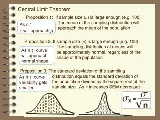
Central Limit Theorem Proposition 1: If sample size (n) is large enough (e.g. 100) The mean of the sampling distribution will approach the mean of the population As n ↑ x will approach µ Proposition 2: If sample size (n) is large enough (e.g. 100) The sampling distribution of means will be approximately normal, regardless of the shape of the population As n ↑ curve will approach normal shape Proposition 3: The standard deviation of the sampling distribution equals the standard deviation of the population divided by the square root of the sample size. As n increases SEM decreases. As n ↑ curve variability gets smaller X X X X X X X X X X X X X X X X X X X X X X X X X X X X X X X X X X X X X X X X X X X X
. Writing Assignment: Writing a letter to a friend • Imagine you have a good friend (pick one). This is a good friend whom you consider to be smart and interested in stuff generally. They are teaching themselves stats (hoping to test out of the class) but need your help on a couple ideas. For this assignment please write your friend/mom/dad/ favorite cousin a letter answering these five questions: (Feel free to use diagrams and drawings if you think that can help) • Dear Friend, • 1. I’m struggling with this whole Central Limit Theorem idea. Could you • describe for me the difference between a distribution of raw scores, and a • distribution of sample means? • 2. I also don’t get the “three propositions of the Central Limit Theorem”. They all • seem to address sample size, but I don’t get how sample size could affect • these three things. If you could help explain it, that would be really helpful.
Let’s try one Types of probability Marietta is a manager of a movie theater. She is trying to figure out whether it is a good idea to install 3-D equipment. It is expensive but she has looked at other (similar) theaters and she is 95% sure that she will make enough money in additional sales to offset her investment. This is an example of a _____ probability. a. Empirical probability b. Classical probability c. Subjective probability d. Not enough information provided Correct Answer
Let’s try one Types of probability Marietta is a manager of a movie theater. She is trying to figure out how much candy (Junior Mints) to stock. She measured the number of boxes of Junior Mints sold for the past 2 months and found that she consistently sold 90% of her stock. She believes that she will sell 90% of her stock of Junior Mints this month. This belief is based on the previous months’ sales. This is an example of a _____ probability. a. Empirical probability b. Classical probability c. Subjective probability d. Not enough information provided Correct Answer
Let’s try one Types of probability Marietta is a manager of a movie theater. She is trying to figure out which employee knows the most about movies. She gives a 100 item test that is made up of all “true” / “false” questions. She believes that even if the employees know absolutely nothing about movie trivia, that they will get 50% right, just by guessing. She knows this even before a single employee takes the test. This is an example of a _____ probability. a. Empirical probability b. Classical probability c. Subjective probability d. Not enough information provided Correct Answer
Types of probability Let’s try one • Frank is a high school physics teacher who also coaches the track team. The track team has been doing very well and have been traveling to competitions a lot. He knows that several of the athletes have missed class because of the excessive traveling. But he also knows they have been working especially hard, and he believes that they will all get above 90% on his next exam. This is an example of a _____ probability. • a. Empirical probability • b. Classical probability • c. Subjective probability • d. Not enough information provided Correct Answer
Let’s try one Types of probability Frank is a high school physics teacher who also coaches the football team. Before each game he tosses a coin to determine which team will kick the ball, and which team will receive. He believes that the “blue” team has a 50% chance of kicking the ball as determined by the coin toss. This is an example of a _____ probability. a. Empirical probability b. Classical probability c. Subjective probability d. Not enough information provided Correct Answer
Let’s try one Types of probability Frank is a high school physics teacher. He has given this same exam every year for 5 years. In every one of those 5 years, 5% of his class failed the exam. Based on these data, he believes that 5% of his current students will probably fail this next exam. This is an example of a _____ probability. a. Empirical probability b. Classical probability c. Subjective probability d. Not enough information provided Correct Answer
Let’s try one According to the Central Limit Theorem, as sample size increases a. variability also increases b. variability decreases c. variability stays the same d. not enough information provided X X X X X X X X X X X X X X X X X X X X X X X X X X X X X X X X X X X X X X X X X X X X
Let’s try one According to the Central Limit Theorem, as sample size increases, the mean of the sampling distribution a. approaches the population mean b. becomes less like the population mean c. is unrelated to the population mean d. not enough information provided X X X X X X X X X X X X X X X X X X X X X X X X X X X X X X X X X X X X X X X X X X X X
Let’s try one According to the Central Limit Theorem, as sample size increases, the shape of the sampling distribution approaches a. the shape of the population b. a normal shape (bell-shaped) c. a skewed shape d. not enough information provided X X X X X X X X X X X X X X X X X X X X X X X X X X X X X X X X X X X X X X X X X X X X
MGMT 276: Statistical Inference in Management. Welcome http://www.thedailyshow.com/video/index.jhtml?videoId=188474&title=an-arab-family-man
Please read: Chapters 5 - 9 in Lind book & Chapters 10, 11, 12 & 14 in Plous book: Lind Chapter 5: Survey of Probability Concepts Chapter 6: Discrete Probability Distributions Chapter 7: Continuous Probability Distributions Chapter 8: Sampling Methods and CLT Chapter 9: Estimation and Confidence Interval Plous Chapter 10: The Representativeness Heuristic Chapter 11: The Availability Heuristic Chapter 12: Probability and Risk Chapter 14: The Perception of Randomness
Use this as your study guide By the end of lecture today3/1/11 Connecting intentions of studies with Experimental Methodologies Appropriate statistical analyses Appropriate graphs Quasi & True Experimental Designs Correlational designs Between and Within participant designs Independent and Dependent Variables Multifactorial designs Graphing Numeric versus Categorical Variables http://www.youtube.com/watch?v=Br6pV1YK6Jg http://today.msnbc.msn.com/id/33411196/ns/today-today_health/
Please click in Homework due next class - (Due March 8th) My last name starts with a letter somewhere between A. A – D B. E – L C. M – R D. S – Z Complete Homework #9Connecting Intention with Design Available on class website Please double check – All cell phones other electronic devices are turned off and stowed away Turn your clicker on
Connecting intentions of studies with Experimental Methodologies Appropriate statistical analyses Appropriate graphs Today I want to present some “typical designs”. We will spend the next couple weeks filling in the details. We’ll come back to these distinctions over and over again, and build on them for the rest of the semester. Let’s get this overview well! Not worry about calculation details for now
Create example of each type Identify IV (one or two) Identify DV (one or two) Draw possible graph for each Writing Assignment Think about this as we work through each type of study Study Type 1: Confidence Intervals Study Type 2: t-test Study Type 3: One-way Analysis of Variance (ANOVA) Study Type 4: Two-way Analysis of Variance (ANOVA) Study Type 5: Correlation Study Type 6: Simple and Multiple regression We’ll come back to these distinctions over and over again, and build on them for the rest of the class. Let’s get this overview well! Not worry about calculation details for now Study Type 7: Chi Square
Remember, this is just introduction to the idea Not worry about calculation details for now, we will get to those soon Study Type 1: Confidence Intervals On average newborns weigh 7 pounds, and are 20 inches long. My sister just had a baby - guess how much it weighs? Makes sense, right?!? Guess the mean. On average you would be right most often if you always guessed the mean Point estimate versus confidence interval: Guessing a single number versus a range of numbers What if you really needed to be right?!!? You could guess a range with smallest and largest possible scores. (how wide a range to be completely sure? Confidence interval: Guessing a range (max and min) and assigning a level of confidence that the score falls in that range
Remember, this is just introduction to the idea Not worry about calculation details for now, we will get to those soon Study Type 1: Confidence Intervals Confidence Intervals: A range of values that, with a known degree of certainty, includes an unknown population characteristic, such as a population mean 100% Confidence Interval: We can be 100% confident that our population mean falls between these two scores (Guess absurdly large and small values) 99% Confidence Interval: We can be 99% confident that our population mean falls between these two scores 95% Confidence Interval: We can be 95% confident that our population mean falls between these two scores Which has a wider interval relative to raw scores 95% or 99%?
Remember, this is just introduction to the idea Not worry about calculation details for now, we will get to those soon Study Type 1: Confidence Intervals Confidence Intervals: A range of values that, with a known degree of certainty, includes an unknown population characteristic, such as a population mean • This sample of 10,000 newborns • a mean weight is 7 pounds. What do you think the minimum and maximum weights would be to capture 95% of all newborns? • This sample of 1000 flights, the mean number of empty seats is 12. What do you think the minimum and maximum number of empty seats are likely to be in the flights today with a 95% level of certainty? • You can use a mean of a sample • to guess the • mean of population • mean of a smaller sample • most likely score for an individual • This sample of 500 households produced • a mean income of $35,000 a year. What do you think the minimum and maximum income levels are so that we are 95% confident that we captured Mabel’s?
Study Type 1: Confidence Intervals Study Type 2: t-test We are looking to compare two means
Study Type 2: t-test analysis Single Independent Variable (categorical) comparing two groups Single Dependent Variable (numerical/continuous) Used to test the effect of the IV on the DV Andrea was interested in the effect of vacation time on productivity of the workers in her department. She randomly assigned workers into two groups, she allowed one group to go on vacation while the other group had no vacation. After the vacation she measured productivity for the two groups. Independent Variable Dependent Variable Between or within Quasi or true Causal relationship? Productivity Yes Vacation No Vacation
Andrea was interested in the effect of vacation time on productivity of the workers in her department. She randomly assigned workers into two groups, she allowed one group to go on vacation while the other group had no vacation. After the vacation she measured productivity for the two groups. This is an example of a true experiment. Dependent variable is always quantitative If “true” experiment (randomly assigned to groups) we can conclude that vacation had an effect - it increased productivity In t-test, independent variable is qualitative (with two groups) If “quasi” experiment (not randomly assigned to groups), we can conclude only that data suggest that vacation may have had an effect; productivity increased for those who went on vacation, but we can’t rule out other explanations.
Study Type 2: t-test analysis Single Independent Variable (categorical) comparing two groups Single Dependent Variable (numerical/continuous) Comparing two means (2 bars on graph) Used to test the effect of the IV on the DV Please note: a t-test allows us to compare two means If the means are statistically different - we say that there is “real” difference that is not just due to chance - we say there is a statistically significant difference p < 0.05 p < 0.05 is most common value – the “p value” can vary (p < 0.01, or p < 0.001)
Study Type 1: Confidence Intervals Study Type 2: t-test Study Type 3: One-way Analysis of Variance (ANOVA) Comparing more than two means
Study Type 3: One-way ANOVA Single Independent Variable comparing more than twogroups Single Dependent Variable (numerical/continuous) Used to test the effect of the IV on the DV Ian was interested in the effect of incentives for girl scouts on the number of cookies sold. He randomly assigned girl scouts into one of three groups. The three groups were given one of three incentives and looked to see who sold more cookies. The 3 incentives were 1) Trip to Hawaii, 2) New Bike or 3) Nothing. This is an example of a true experiment How could we make this a quasi-experiment? Independent Variable: Type of incentive Levels of Independent Variable: None, Bike, Trip to Hawaii Dependent Variable: Number of cookies sold Levels of Dependent Variable: 1, 2, 3 up to max sold Between participant design Causal relationship: Incentive had an effect – it increased sales
Study Type 3: One-way ANOVA Single Independent Variable comparing more than two groups Single Dependent Variable (numerical/continuous) Used to test the effect of the IV on the DV Ian was interested in the effect of incentives for girl scouts on the number of cookies sold. He randomly assigned girl scouts into one of three groups. The three groups were given one of three incentives and looked to see who sold more cookies. The 3 incentives were 1) Trip to Hawaii, 2) New Bike or 3) Nothing. This is an example of a true experiment Dependent variable is always quantitative Sales Sales New Bike None Trip Hawaii New Bike None Trip Hawaii In an ANOVA, independent variable is qualitative (& more than two groups)
Study Type 1: Confidence Intervals Study Type 2: t-test Study Type 3: One-way Analysis of Variance (ANOVA) Study Type 4: Two-way Analysis of Variance (ANOVA) Comparing two independent variables Each one has multiple levels
“Two-way” = “Two IVs” Study Type 4: Two-way ANOVA Ian was interested in the effect of incentives (and age) for girl scouts on the number of cookies sold. He randomly assigned girl scouts into one of three groups. The three groups were given one of three incentives and he looked to see who sold more cookies. The 3 incentives were: 1) Trip to Hawaii, 2) New Bike or 3) Nothing. He also measured the scouts’ ages. Independent Variable #1 Independent Variable #2 Dependent Variable
Study Type 4: Two-way ANOVA Multiple Independent Variables (categorical), each variable comparing two or moregroups Single Dependent Variable (numerical/continuous) Used to test the effect of two IV on the DV Independent Variable #1: Type of incentive Levels of Independent Variable: None, Bike, Trip to Hawaii Independent Variable #2: Age Levels of Independent Variable: Elementary girls versus college Dependent Variable: Number of cookies sold Levels of Dependent Variable: 1, 2, 3 up to max sold Between participant design Results: Incentive had an effect – it increased sales Data suggest age had an effect – older girls sold more
Study Type 4: Two-way ANOVA Two Independent Variables (categorical) Single Dependent Variable (numerical/continuous) Used to test the effect of two IV on the DV Dependent variable is always quantitative College College Elementary Sales Elementary Sales New Bike None Trip Hawaii New Bike None Trip Hawaii In an ANOVA, both independent variables are qualitative (with more than two groups)
Study Type 1: Confidence Intervals Study Type 2: t-test Study Type 3: One-way Analysis of Variance (ANOVA) Study Type 4: Two-way Analysis of Variance (ANOVA) Study Type 5: Correlation
Pretty much all correlations are “quasi-experimental” Study Type 5: Correlation plots relationship between two continuous / quantitative variables Neutral relative to causality – but especially useful for predictions Relationship between amount of money spent on advertising and amount of money made in sales Dependent variable is always quantitative Dollars spent on Advertising Positive Correlation In correlation, both variables are quantitative Dollars in Sales Describe strength and direction of correlation – in this case positive/strong Graphing correlations use scatterplots (not bar graphs)
Study Type 1: Confidence Intervals Study Type 2: t-test Study Type 3: One-way Analysis of Variance (ANOVA) Study Type 4: Two-way Analysis of Variance (ANOVA) Study Type 5: Correlation Study Type 6: Simple and Multiple regression
YearlyIncome Expenses per year Study Type 6: Regression: Using the correlation to predict the value of one variable based on its relationship with the other variable Multiple regression will use multiple independent variables to predict the dependent variable You probably make this much The predicted variable goes on the “Y” axis and is called the dependent variable. The predictor variable goes on the “X” axis and is called the independent variable You probably make this much Dependent Variable (Predicted) If you spend this much If you save this much Independent Variable 1 (Predictor) If you spend this much Independent Variable 2 (Predictor)
Study Type 1: Confidence Intervals Study Type 2: t-test Study Type 3: One-way Analysis of Variance (ANOVA) Study Type 4: Two-way Analysis of Variance (ANOVA) Study Type 5: Correlation Study Type 6: Simple and Multiple regression Study Type 7: Chi Square
Study Type 7: Chi square is used to evaluate nominal data (just count how many in each category) or objects or events Variables are nominal or ordinal (so we comparing frequencies, not means) What is most popular ride at Disneyland? Just count how many people ride each one. a. Dumbob. Peter Panc. Space Mountaind. Splash Mountaine. Small World We could gather this data using clickers
Let’s try one What type of analysis is this? Marietta is a manager of a movie theater. She wanted to know whether there is a difference in concession sales for afternoon (matinee) movies vs. evening movies. She took a random sample of 25 purchases from the matinee movie (mean of $7.50) and 25 purchases from the evening show (mean of $10.50). She compared these two means. This is an example of a _____. a. correlation b. t-test c. one-way ANOVA d. two-way ANOVA t-test Let’s try another one This is an example of a a. between participant design b. within participant design c. mixed participant design Between
Thank you! See you next time!!