Categorical Data Analysis PGRM 14
Categorical Data Analysis PGRM 14. What is categorical data?. The measurement scale for the response consists of a number of categories. Data Analysis considered:. Response variable(s) is categorical Explanatory variable(s) may be categorical or continuous.

Categorical Data Analysis PGRM 14
E N D
Presentation Transcript
What is categorical data? The measurement scale for the responseconsists of a number of categories
Data Analysis considered: • Response variable(s)is categorical • Explanatory variable(s) may be categorical or continuous Example: Does Post-operative survival (categorical response) depend on the explanatory variables? Sex (categorical) Age (continuous) Example: In a random sample of Irish farmers is there a relationship between attitudes to the EU and farm system. Farm system (categorical) Attitude to EU (categorical/ordinal)? (Two response variables - no explanatory variables) Could one of these be regarded as explanatory?
Measurementscales for categorical data Nominal - no underlying order Ordinal - underlying orderin the scale Interval - underlying numerical distance between scale points
Tables reporting count data: single level Example:A geneticist carries out a crossing experiment between F1 hybrids of a wild type and a mutant genotype and obtains an F2 progeny of 90 offspring with the following characteristics. Evidence that a wild type is dominant, giving on average 8:1 offspring phenotype in its favour?
Tables for count data: two-way Example:A sample 124 mice was divided into two groups, 84 receiving a standard dose of pathogenic bacteria followed by an antiserum and a control group of 40 not receiving the antiserum. After 3 weeks the numbers dead and alive in each group were counted. Association betweenmortality and treatment?
Tables for count data: two-way Example (Snedecor & Cochran):The table below shows the number of aphids alive and dead after spraying with four concentrations of solutions of sodium oleate. • Has the higher concentration given a significantly different percentage kill? • Is there a relationship between concentration and mortality?
Is this the relationship? Note:categorical responseinterval categorical explanatory variable ?
Tables for count data: two-way Example (Cornfield 1962)Blood pressure (BP) was measured on a sample of males aged 40-59, who were also classified by whether they developed coronary heart disease (CHD) in a 6-year follow-up period.BP:interval categorical variablein 8 classes CHD:CHD or No-CHD • Is the incidence of CHD independent of BP? • Is there a simple relationship between the probability of CHD and the level of BP?
3-way table Example: Grouped binomial (response has 2 categories) data - patterns of psychotropic drug consumption in a sample from West London (Murray et al 1981, Psy Med 11,551-60)
Non-tabulated data Example: Individual Legousia plants were monitored in an experiment to see whether they survived after 3 months.Survived -yes is scored 1 Survived -no scored 0.Also recorded were: CO2 treatment – 2 levels low and high Density of Legousia Density of companion species Height of the plant (mm)two weeks after planting. Most individuals will have a unique profile in these three additional variables and so tabulation of the data by them is not feasible. The individual data is presented
Non-tabulated data • Is survival related to the explanatory variables:CO2, Height, density-self, density-companions? • Can the probability of survival be predicted from the subject’s profile? Response
Fixed and non-fixed margins • One margin fixed: Samples of fixed size are selected for one or more categories and individuals are classified by the other category(s). • No margin fixed: Individuals in a single sample are simultaneously classified by several categorical variables. Difference between these depends on the experimental design and how this specified the data should be collected. Method of analysis is the same.
Asking the right question • Data summarized by counts • Questions usually relate to %s(equivalently proportions)
Hypotheses for Categorical Data • Categorical data is summarised by counting individuals falling into the various combinations of categories • Hypotheses relate to:the probability of an individual being in a particular category • These probabilities are estimated by the observed proportions in the data • Using a sample proportion, p, from a sample of size n, to estimate a population proportion the standard error is √(p(1 – p)/n)egwith p = 0.5, n = 1100, 2×SE = 0.03the often mentioned 3% margin of error
Example Does % dead depend on antiserum? • Equivalently: • Is there an association between mortality and antiserum? • Is mortality independent of anitserum?
Example • As usual we set up a null hypothesis and measure the extent to which the data conflicts with this • Here H0: prob of death for anti = prob of death for control • equivalently H0: • no association between mortality and antiserum • Mortality and antiserum are independent
Example Expected counts when H0 is true: The overall % dead (37/124)would apply to antiserum & control For the 84 antiserum this would give(84×37)/124 dead and (84×87)/124 alive For the 40 control this would give(40×37)/124 dead and (40×87)/124 alive E = (row total)(column total)/(table total)
Observed and expected counts Observed Expected Note: some rounding error
Chi-squared statistic : X2 • X2 measures difference between observed counts, O, and expected (when H0 holds) counts, E • If LARGE provides evidence against H0, ie evidence for an association (dependence) of mortality on anitserum. • X2 = ∑(O – E)2/E • Here SAS/FREQ gives: X2 = 6.48 p = Prob(X2 > 6.48 when H0 is true) = 0.0109 • Conclusion:there is evidence (p < 0.05) that mortality depends on antiserum
Practical Exercise Use Excel to calculate X2 and p Lab Session 5 exercise 5.1 (a)
SAS/FREQ OUTPUT Description of cell contents X2 = ∑(O – E)2/E O = Frequency E = Expected Row Percents make most sense here(% alive/dead in each antiserum group)
SAS/FREQ OUTPUT DF = (r–1)×(c-1) X2 = ∑(O – E)2/E Ignore!
Area 0.05 6.48 P = 0.001 with X2 = 6.48 Area0.001 68% values < 1(not shown)
Aphid example (SAS/FREQ OUTPUT) X2 = 17.18p = 0.0007 (3 df) Note the largest contributions (O – E)2/E to X2 (8.96 & 3.87) are in top corners
Locating the concentration effect X2 = 0.99p = 0.32 X2 = 2.71p = 0.10
Locating the concentration effect X2 = 12.83p = 0.0003
SAS – data format for FREQ procedure 2 cols identify the cell Final column is the ‘response’– the frequency count for the cell Conc status number 0.65 d 55 0.65 a 22 1.10 d 62 1.10 a 13 1.60 d 100 1.60 a 12 2.10 d 72 2.10 a 5
Validity of chi-squared (2) test • Test is based on an approximation leading to use of the 2 distribution to calculate p-values • With several DF and E 5 approximation is ok • If E < 1 in any cell approximation may be bad • With a number of cells in the table perhaps a third or quarter can have E between 1 & 5 without serious departures from 2 based p-values. (PGRM pg 14-11) • In cases where good approximation is in doubt use Fisher’s exact test (SAS/FREQ tables option exact)
Code: SAS/FREQ procfreqdata = conc;weight number;tables status*conc / chisq cellchi2 expected norow nopercent nocum;quit;
Practical Exercise SAS/FREQ procedure Lab Session 5 exercise 5.1 (b) – (d)
Is this the relationship? Note:categorical responseinterval categorical explanatory variable ?
Why logistic and not just 2? • For sparse data(eg where individuals will have unique profiles) • With many categorical explanatory variables • With quantitative explanatory variables In the case of a continuous response we have looked to see if the mean, , can be expressed as = a + bx With categorical data we want an expression for p (the probability of the response in one of the 2 response categories) butp = a + bxmay give values outside the range 0 to 1!eg p = 0.1 + 0.2x gives p = 1.1 for x = 5
A solution: TRANSFORM • Use the transformation:p = exp(a + bx)/(1 + exp(a + bx)) • i.e. log(p/(1 – p)) = a + bxlog(Odds) = a + bxwhere Odds = p/(1 – p) Note: exp(x) = ex Plot is for: a = 0, b = 1 LOGIT:logit(p) = log(p/(1-p))
SAS/GPLOT logit(p) = −0.119 + 1.25 conc
LD50 – lethal dose for 50% • p = 0.5 • p /(1 – p) = 1 • logit(p) = 0 (since log(1) = 0, WNF!) • 0 = −0.119 + 1.25 conc • conc = 0.119/1.25 = 0.095 log(a) – log(b) = log(a/b) Odd Ratio (OR) Increasing conc by 1% increases logit(p) by 1.25 log(Odds2) – log(Odds1) = 1.25 log(OR) = 1.25 OR = exp(1.25) = 3.49
SAS/GENMOD procgenmoddata = log;model dead/total = conc / predlink = logitdist = binomial;outputout = ppredicted = p;run; conc dead total 0.65 53 771.10 57 751.60 95 1122.10 73 77
Practical Exercise SAS/GENMOD of Logistic Regression Lab Session 5 exercise 5.2 (a) – (g)
Stability analysis (Ex 2 pg 14-15) Heights, diameter and whether they fell over were recorded for 545 plants. Aim: model the probability of stability (not falling over) as a function of height an diameter. Explanatory terms • Model 1:h d h2 d2 hdhopefully high order terms will not be needed! • Model 2:h/d2biologist suggests this!
Model 1: h, d, h2, d2, hd How can I describe this!
Model 2: h/d2 Can understand & even plot this!
SAS/GRAPH But!
Poisson Regression For count data- where eg we count all – not a subset out of a total To estimate the mean, μ, and its relationship with an explanatory variable x use a log link (usually): log(μ) = a + bx ieμ = exp(a + bx) (which will be >0) = ea ebx model count = x / link = log distribution = poisson; SAS/GENMOD
Example: Horseshoe crabs & satellites Each female crab had an attached male (in her nest) & other males (satellites) residing nearby. • Data recorded • No satellites (response) • Color (light medium, medium, dark medium, dark) • Spine condition(both good, one worn/broken, both worn/broken) • Carapace width (cm) • Weight (kg) • Poisson Models: • Log link: log(μ) = a + bx • Identity link: μ = a + bx

