Categorical Data Analysis
Explore the analysis of categorical data in 2x2 contingency tables, measuring risk associations, and interpreting results using relative risk, odds ratio, and absolute risk. Case examples demonstrate application and interpretation in medical research studies.


Categorical Data Analysis
E N D
Presentation Transcript
Categorical Data Analysis • Independent (Explanatory) Variable is Categorical (Nominal or Ordinal) • Dependent (Response) Variable is Categorical (Nominal or Ordinal) • Special Cases: • 2x2 (Each variable has 2 levels) • Nominal/Nominal • Nominal/Ordinal • Ordinal/Ordinal
Contingency Tables • Tables representing all combinations of levels of explanatory and response variables • Numbers in table represent Counts of the number of cases in each cell • Row and column totals are called Marginal counts
Example – EMT Assessment of Kids • Explanatory Variable – Child Age (Infant, Toddler, Pre-school, School-age, Adolescent) • Response Variable – EMT Assessment (Accurate, Inaccurate) Source: Foltin, et al (2002)
2x2 Tables • Each variable has 2 levels • Explanatory Variable – Groups (Typically based on demographics, exposure, or Trt) • Response Variable – Outcome (Typically presence or absence of a characteristic) • Measures of association • Relative Risk (Prospective Studies) • Odds Ratio (Prospective or Retrospective) • Absolute Risk (Prospective Studies)
Relative Risk • Ratio of the probability that the outcome characteristic is present for one group, relative to the other • Sample proportions with characteristic from groups 1 and 2:
Relative Risk • Estimated Relative Risk: 95% Confidence Interval for Population Relative Risk:
Relative Risk • Interpretation • Conclude that the probability that the outcome is present is higher (in the population) for group 1 if the entire interval is above 1 • Conclude that the probability that the outcome is present is lower (in the population) for group 1 if the entire interval is below 1 • Do not conclude that the probability of the outcome differs for the two groups if the interval contains 1
Example - Coccidioidomycosis and TNFa-antagonists • Research Question: Risk of developing Coccidioidmycosis associated with arthritis therapy? • Groups: Patients receiving tumor necrosis factor a (TNFa) versus Patients not receiving TNFa (all patients arthritic) Source: Bergstrom, et al (2004)
Example - Coccidioidomycosis and TNFa-antagonists • Group 1: Patients on TNFa • Group 2: Patients not on TNFa Entire CI above 1 Conclude higher risk if on TNFa
Odds Ratio • Odds of an event is the probability it occurs divided by the probability it does not occur • Odds ratio is the odds of the event for group 1 divided by the odds of the event for group 2 • Sample odds of the outcome for each group:
Odds Ratio • Estimated Odds Ratio: 95% Confidence Interval for Population Odds Ratio
Odds Ratio • Interpretation • Conclude that the probability that the outcome is present is higher (in the population) for group 1 if the entire interval is above 1 • Conclude that the probability that the outcome is present is lower (in the population) for group 1 if the entire interval is below 1 • Do not conclude that the probability of the outcome differs for the two groups if the interval contains 1
Example - NSAIDs and GBM • Case-Control Study (Retrospective) • Cases: 137 Self-Reporting Patients with Glioblastoma Multiforme (GBM) • Controls: 401 Population-Based Individuals matched to cases wrt demographic factors Source: Sivak-Sears, et al (2004)
Example - NSAIDs and GBM Interval is entirely below 1, NSAID use appears to be lower among cases than controls
Absolute Risk • Difference Between Proportions of outcomes with an outcome characteristic for 2 groups • Sample proportions with characteristic from groups 1 and 2:
Absolute Risk Estimated Absolute Risk: 95% Confidence Interval for Population Absolute Risk
Absolute Risk • Interpretation • Conclude that the probability that the outcome is present is higher (in the population) for group 1 if the entire interval is positive • Conclude that the probability that the outcome is present is lower (in the population) for group 1 if the entire interval is negative • Do not conclude that the probability of the outcome differs for the two groups if the interval contains 0
Example - Coccidioidomycosis and TNFa-antagonists • Group 1: Patients on TNFa • Group 2: Patients not on TNFa Interval is entirely positive, TNFa is associated with higher risk
Fisher’s Exact Test • Method of testing for association for 2x2 tables when one or both of the group sample sizes is small • Measures (conditional on the group sizes and number of cases with and without the characteristic) the chances we would see differences of this magnitude or larger in the sample proportions, if there were no differences in the populations
Example – Echinacea Purpurea for Colds • Healthy adults randomized to receive EP (n1.=24) or placebo (n2.=22, two were dropped) • Among EP subjects, 14 of 24 developed cold after exposure to RV-39 (58%) • Among Placebo subjects, 18 of 22 developed cold after exposure to RV-39 (82%) • Out of a total of 46 subjects, 32 developed cold • Out of a total of 46 subjects, 24 received EP Source: Sperber, et al (2004)
Example – Echinacea Purpurea for Colds • Conditional on 32 people developing colds and 24 receiving EP, the following table gives the outcomes that would have been as strong or stronger evidence that EP reduced risk of developing cold (1-sided test). P-value from SPSS is .079.
McNemar’s Test for Paired Samples • Common subjects being observed under 2 conditions (2 treatments, before/after, 2 diagnostic tests) in a crossover setting • Two possible outcomes (Presence/Absence of Characteristic) on each measurement • Four possibilities for each subjects wrt outcome: • Present in both conditions • Absent in both conditions • Present in Condition 1, Absent in Condition 2 • Absent in Condition 1, Present in Condition 2
McNemar’s Test for Paired Samples • H0: Probability the outcome is Present is same for the 2 conditions • HA: Probabilities differ for the 2 conditions (Can also be conducted as 1-sided test)
Example - Reporting of Silicone Breast Implant Leakage in Revision Surgery • Subjects - 165 women having revision surgery involving silicone gel breast implants • Conditions (Each being observed on all women) • Self Report of Presence/Absence of Rupture/Leak • Surgical Record of Presence/Absence of Rupture/Leak Source: Brown and Pennello (2002)
Example - Reporting of Silicone Breast Implant Leakage in Revision Surgery • H0: Tendency to report ruptures/leaks is the same for self reports and surgical records • HA: Tendencies differ
Pearson’s Chi-Square Test • Can be used for nominal or ordinal explanatory and response variables • Variables can have any number of distinct levels • Tests whether the distribution of the response variable is the same for each level of the explanatory variable (H0: No association between the variables • r = # of levels of explanatory variable • c = # of levels of response variable
Pearson’s Chi-Square Test • Intuition behind test statistic • Obtain marginal distribution of outcomes for the response variable • Apply this common distribution to all levels of the explanatory variable, by multiplying each proportion by the corresponding sample size • Measure the difference between actual cell counts and the expected cell counts in the previous step
Pearson’s Chi-Square Test • Notation to obtain test statistic • Rows represent explanatory variable (r levels) • Cols represent response variable (c levels)
Pearson’s Chi-Square Test • Marginal distribution of response and expected cell counts under hypothesis of no association:
H0: No association between variables HA: Variables are associated Pearson’s Chi-Square Test
Example – EMT Assessment of Kids Observed Expected
Example – EMT Assessment of Kids • Note that each expected count is the row total times the column total, divided by the overall total. For the first cell in the table: • The contribution to the test statistic for this cell is
Example – EMT Assessment of Kids • H0: No association between variables • HA: Variables are associated Reject H0, conclude that the accuracy of assessments differs among age groups
Ordinal Explanatory and Response Variables • Pearson’s Chi-square test can be used to test associations among ordinal variables, but more powerful methods exist • When theories exist that the association is directional (positive or negative), measures exist to describe and test for these specific alternatives from independence: • Gamma • Kendall’s tb
Concordant and Discordant Pairs • Concordant Pairs - Pairs of individuals where one individual scores “higher” on both ordered variables than the other individual • Discordant Pairs - Pairs of individuals where one individual scores “higher” on one ordered variable and the other individual scores “higher” on the other • C = # Concordant Pairs D = # Discordant Pairs • Under Positive association, expect C > D • Under Negative association, expect C < D • Under No association, expect C D
Example - Alcohol Use and Sick Days • Alcohol Risk (Without Risk, Hardly any Risk, Some to Considerable Risk) • Sick Days (0, 1-6, 7) • Concordant Pairs - Pairs of respondents where one scores higher on both alcohol risk and sick days than the other • Discordant Pairs - Pairs of respondents where one scores higher on alcohol risk and the other scores higher on sick days Source: Hermansson, et al (2003)
Example - Alcohol Use and Sick Days • Concordant Pairs: Each individual in a given cell is concordant with each individual in cells “Southeast” of theirs • Discordant Pairs: Each individual in a given cell is discordant with each individual in cells “Southwest” of theirs
Measures of Association • Goodman and Kruskal’s Gamma: • Kendall’s tb: When there’s no association between the ordinal variables, the population based values of these measures are 0. Statistical software packages provide these tests.