Introduction to Categorical Data Analysis
Introduction to Categorical Data Analysis. KENNESAW STATE UNIVERSITY STAT 8310. Introduction. The ‘General Linear Model’ (AKA as Normal Theory Methods) Linear Regression Analysis The Analysis of Variance These methods are appropriate for analyzing data with:

Introduction to Categorical Data Analysis
E N D
Presentation Transcript
Introduction to Categorical Data Analysis KENNESAW STATE UNIVERSITY STAT 8310
Introduction • The ‘General Linear Model’ (AKA as Normal Theory Methods) • Linear Regression Analysis • The Analysis of Variance • These methods are appropriate for analyzing data with: • A quantitative (or continuous) response variable • Quantitative and/or categorical explanatory variables
Example of a Typical Regression • EXAMPLE: Predicting the Blood Pressure (measured in mmHg)from Cholesterol level (measured in mg/dL) & smoking status (smoker, non-smoker) • mmHg = millimeters of mercury • mg/dL = milligrams of cholesterol per deciliter
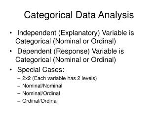
Introduction • Categorical Data Analysis (CDA) involves the analysis of data with a categorical response variable. • Explanatory variables can be either categorical or quantitative.
Example of CDA • EXAMPLE: Predicting the presence of heart disease (yes, no) from Cholesterol level (measured in mg/dL) & smoking status (smoker, non-smoker)
Quantitative Variables • A quantitative variable • measures the quantity or magnitude of a characteristic or trait possessed by an experimental unit. • has well defined units of measurement. • often answer the question, ‘how much?’. • Sometimes referred to as a continuous variable.
Quantitative Variables • What are some examples of quantitative explanatory variables? • What are some examples of quantitative response variables?
Categorical Variables • A categorical variable • has a measurement scale consisting of a set of categories • places or identifies experimental units as belonging to a particular group or category • Sometimes referred to as a qualitative or discrete variable.
Categorical Variables • What are some examples of categorical explanatory variables? • What are some examples of categorical response variables?
Types of Categorical Variables • Dichotomous (AKA Binary) • Categorical variables with only 2 possible outcomes • EXAMPLE: Smoker (yes, no) • Polychotomous or Polytomous • Categorical variables with more than 2 possible outcomes • EXAMPLE: Race (Caucasian, African American, Hispanic, Other)
Another Dimension of Polytomous Categorical Variables • Nominal • Are those that merely place experimental units into unordered groups or categories. • EXAMPLE: • Favorite Music (classical, rock, jazz, opera, folk)
Another Dimension of Polytomous Categorical Variables • Ordinal • Categorical variables whose values exhibit a natural ordering. • EXAMPLE: • Prognosis (poor, fair, good, excellent)
Summarizing Categorical Variables • Often times in CDA, it is possible to fully analyze data using a summarization of the data (the raw data is many times not necessary!). • Therefore, in CDA we make the distinction between raw data and grouped data.
Summarizing Categorical Variables • A natural way to summarize categorical variables is raw counts or frequencies. • A frequency table summarizes the raw counts of 1 categorical variable. • A contingency table summarizes the raw counts of 2 or more categorical variables.
Summarizing Categorical Variables • Along with frequencies, we also often summarize categorical variables with: • Proportions • Percentages
Summarizing Categorical Variables • Example of some raw data: • What kind of variable is Final Exam Grade?
Summarizing Categorical Variables • Example of a frequency table for these data is:
Summarizing Categorical Variables 2 • Example of some raw data:
Summarizing Categorical Variables 2 • Example of a contingency table for these data is:
Summarizing Categorical Variables 2 • Traditionally, when summarizing explanatory & response variables in a contingency table, the explanatory variables are expressed in rows, and the response variables in columns.
Summarizing Categorical Variables • Graphical means for summarizing categorical variables include pie charts and bar charts.
Probability Distributions • In typical linear regression, we assume that the response variable is normally distributed and therefore use the normal distribution during hypothesis testing.
Probability Distributions • In CDA, we use: • The Binomial Distribution • For dichotomous variables • The Multinomial Distribution • For polytomous variables • The Poisson Distribution • For polytomous variables
The Binomial Distribution • Appropriate when there are: • n independent and identical trials • 2 possible outcomes (generically named “success” & “failure”)
The Binomial PMF • PMF = Probability Mass Function • Gives the probability of outcome y for Y • Y ~ Bin(n, π)
A Review of Combinations and Factorials • nCy • The Binomial Coefficient – counts the total number of ways one could obtain y successes in n trials.
A Review of Combinations and Factorials • Factorials – n! • is the product of all positive integers less than or equal to n. • 0! = 1 • 1! = 1 • Example: • 4! = 4 x 3 x 2 x 1 = 24
Example Problem • A coin is tossed 10 times. Let Y = the number of heads. • Use statistical notation to specify the distribution of Y. • Find the mean [E(Y)] and standard deviation of Y [σ(Y)] • What is the P(Y = 8)?
The Multinomial Distribution • Used for modeling the distribution of polytomous variables
Example Problem • Researchers categorize the outcomes from a particular cancer treatment into 3 groups (no effect, improvement, remission). Suppose (π1, π2,π3) = (.20, .70, .10). • Show all possible outcomes if n = 2. • Find the multinomial probability that (n1, n2, n3) = (2,6,1).
Overview of CDA Methods • Contingency Table Analysis • Logistic Regression (AKA Logit Models) • Multicategory Logit Models • Loglinear Models
Contingency Table Analysis • The historical method for analyzing CD • Involves constructing a n-way contingency table (where n = the number of categorical variables)
Contingency Table Analysis We use contingency table analysis for the following: • Identify the presence of an association • The hypothesis test of independence • Measure or gauge the strength of an association
Logistic Regression (AKA Logit Models) • We use Logit Models to: • Analyze data with a dichotomous response variable • A single or multiple categorical and/or continuous explanatory variables
Multicategory Logit Models • We use Multicategory Logit Models to: • Analyze data with a polytomous response variable • A single or multiple categorical and/or continuous explanatory variables
Loglinear Models • We use Loglinear Models to analyze data: • with a polytomous response variable • OR • with multiple response variables • OR • where the distinction between explanatory and response variable is not clear & 1 or more of those variables is polytomous • Often associated with the analysis of count data
Review of 1 Proportion Hypothesis Tests • MOTIVATING EXAMPLE: • National data in the 1960s showed that about 44% of the adult population had never smoked cigarettes. In 1995, a national health survey interviewed a random sample of 881 adults and found that 414 had never been smokers. Has the percentage of adults who never smoked increased?
Review of 1 Proportion Hypothesis Tests • STEPS: • Gather information • Check assumptions • Compute Tn & obtain p-value • Make conclusions
Review of 1 Proportion Hypothesis Tests • ANSWER: • There is sufficient statistical evidence to reject the null hypothesis and conclude that the proportion of adults who have never smoked has increased; z = 1.789, p = .036.
Review of Confidence Intervals for Proportions • MOTIVATING EXAMPLE: • Construct a 99% Confidence Interval for the true population of adult non-smokers based on this sample data.
Review of Confidence Intervals for Proportions • ANSWER: • We are 99% confident that the interval from .427 to .513 contains the true proportion of adults who have never smoked.
Review of Confidence Intervals for Proportions • ANSWER: • We are 99% confident that the interval from .427 to .513 contains the true proportion of adults who have never smoked.
Class Activity 1 • Go to the course website at: http://www.science.kennesaw.edu/~dyanosky/stat8310.html • Navigate to the ‘Class Activities’ Page. • Complete CA.1
Solutions to Class Activity 1 (#1) • We reject the null hypothesis at the α = .05 level and conclude that percent of non-compliant vehicles has increased; z = 2.38, p = .009. • We are 90% confident that the interval from .147 to .235 contains the true proportion of non-compliant vehicles.
Solutions to Class Activity 1 (#2) • We fail to reject the null hypothesis at the α = .01 level. There is insufficient evidence to conclude that the population proportion of smokers has changed; z = -1.78, p = .075. • We are 95% confident that the interval from .497 to .563 contains the true proportion of adults who currently smoke.

