Download

1 / 18
180 likes | 301 Vues
Immune Cells Detection of the In Vivo Rejecting Heart in USPIO-Enhanced MRI. Hsun-Hsien Chang 1 , Jos é M. F. Moura 1 , Yijen L. Wu 2 , and Chien Ho 2 1 Department of Electrical and Computer Engineering 2 Pittsburgh NMR Center for Biomedical Research

E N D
Immune Cells Detection of the In Vivo Rejecting Heart in USPIO-Enhanced MRI Hsun-Hsien Chang1, José M. F. Moura1, Yijen L. Wu2, and Chien Ho2 1Department of Electrical and Computer Engineering 2Pittsburgh NMR Center for Biomedical Research Carnegie Mellon University, Pittsburgh, PA, USA Work supported by NIH grants (R01EB/AI-00318 and P4EB001977)
Research Motivation • The extreme treatment of the heart failure is transplantation. • Gold standard diagnosis method (i.e., biopsy) of heart rejection • is invasive. • is prone to sampling errors. • Alternative diagnosis method: contrast-enhanced cardiac MRI • is non-invasive. • monitors the wholein vivo heart.
RV LV rejecting tissue Mechanism of Contrast-Enhanced MRI • immune cells (e.g. macrophages). • contrast agents (USPIO, ultra-small super-paramagnetic iron oxide) label the immune cells • High relaxivity causes low image intensities under T2* weighted MRI.
Immune Cells Classification: Challenges Identify immune cells (i.e., dark pixels): • Large number of myocardial pixels • Manual classification is labor-intensive and time consuming. • Dispersion of immune cells • Immune cells accumulate in multiple regions without known patterns. • Heart motion blurs images • It is hard to distinguish the boundaries between the USPIO-labeled and unlabeled pixels Post Operation Day (POD) 3. • Need an automatic algorithm to classify pixels as USPIO-labeled or unlabeled. POD 5.
Immune Cells Classification: Overview • Main idea: • Partition the image into USPIO-labeled and unlabeled parts. • Graph theory approach: • Describe the image as a graph. • Find the optimal edge cut.
Outline • Introduction • Methodology: Graph Partitioning • Graph Representation of the USPIO Image • Optimal Edge Cut and the Cheeger Constant • Optimal Classifier via Optimization • Results and Conclusions
Immune Cells Classification: Algorithm Graph Representation of the USPIO Image Classification through an Edge Cut Optimal Cut from the Cheeger Constant Optimal Classifier via Energy Minimization Red dots are the automatically selected USPIO-labeled pixels.
(a) 0.61 (b) 0.89 (c) 0.76 (d) 0.61 Graph Representation of the USPIO Image Classification through an Edge Cut (e) 0.46 (f) 1.00 (g) 0.62 (h) 0.51 Optimal Cut from the Cheeger Constant (i) 0.23 (j) 0.79 (k) 0.38 (l) 0.43 Optimal Classifier via Energy Minimization (m) 0.00 (n) 0.17 (o) 0.09 (p) 0.28 • Graph: G(V, E). • a set V of vertices representing pixels. • a set E of edges linking the vertices according to a prescribed way. • Edge assignment strategies: • Geographical neighborhood • Feature similarities
Edge cut: • Partition: Graph Representation of the USPIO Image Classification through an Edge Cut Optimal Cut from the Cheeger Constant Optimal Classifier via Energy Minimization • Classification of the pixels into USPIO-labeled or unlabeled is equivalent to partitioning the graph into two disjoint subgraphs. • Graph partitioning: • Divide the vertex set V into disjoint subsets S and S’. • Remove a set of edges, denoted as Edge(S, S’), to make S and S’ disconnected.
8 (a) (b) (2+5+3) X(S) = Graph Representation of the USPIO Image 8 (a) (b) (2+10)c+(10+5+3)d 5 3 2 = 0.33 8 (a) (b) 3 (c) (d) 2 • Consider this example: 10 5 5 Classification through an Edge Cut (c) (d) (8+5+10) 3 2 10 X(S) = (8+5+2)a+(2+10)c (c) (d) 10 = 0.85 Optimal Cut from the Cheeger Constant 8 (a) (b) 8 (a) (b) Optimal Classifier via Energy Minimization 5 5 3 2 2 3 (c) (d) (c) (d) 10 10 (2+5+8+3+10) (8+3+10+2) X(S) = X(S) = (2+10)c+(8+3)b (8+3)b+(2+10)c = 1.21 = 1.00 • Cheeger constant: • Assuming that Vol(S) < Vol(S’). • |Edge(S, S’)| = sum of the edges in the cut. • Vol(S) = sum of edges emanating from all the vertices in S.
+1 0 -1 (c) (d) Graph Representation of the USPIO Image 8 (a) (b) (a) (b) 3 2 5 Classification through an Edge Cut (c) (d) 10 • Derive an objective functional from the Cheeger constant: Optimal Cut from the Cheeger Constant Optimal Classifier via Energy Minimization • Optimal classifier: • Classifier • Classifier
Outline • Introduction • Methodology: Graph Partitioning • Graph Representation of the USPIO Image • Optimal Edge Cut and the Cheeger Constant • Optimal Classifier via Optimization • Results and Conclusions
Heart Rejection at Different Rejection Stages RV Post Operation Day (POD) 3 POD 4 LV RV LV POD 5 POD 6 RV LV RV LV (Data were presented in Wu et al, PNAS 2006)
POD3 POD4 POD5 POD6 POD7 Classification Results Fig1: USPIO-enhanced images Fig2: manual classification (presented in Wu et al, PNAS 2006) Fig3: automatic classification
Immune Cell Accumulation vs. POD Immune cell accumulation area Immune cell accumulation percentage
Conclusions • Develop a graph theoretical approach to classifying immune cells in the USPIO-enhanced images • Represent an image by a graph. • Consider the Cheeger constant for the optimal cut. • Adopt the optimization to find the classifier.
1. Assign edges to the neighboring pixels. (a) 0.61 (b) 0.89 (c) 0.76 (d) 0.61 (e) 0.46 (f) 1.00 (g) 0.62 (h) 0.51 2. Assign edges to similar pixels ( d < 0.1). (i) 0.23 (j) 0.79 (k) 0.38 (l) 0.43 (m) 0.00 (n) 0.17 (o) 0.09 (p) 0.28 Weighted Graph Representation of Image 3. Repeat the procedure to all other pixels.