Download
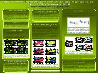
1 / 1
10 likes | 115 Vues

E N D
Figure 3. Box-and-whisker plots of the daily mean temperature distribution in 1970-1999 (a) and in 2070-2099 (b) over the region indicated by a rectangle, respectively in Figure 2d and 2f. Fat white box represents the entire winter season distribution and colored boxes show the distributions inside the four weather regimes. The horizontal line within the box is the median; lower and upper box bounds show the 25th and 75th percentiles, respectively; lower and upper whisker bounds indicate the 5th and 95th percentiles, respectively. Color legend is as in Figure 2. Units are in °C. Figure 4. Mean winter temperature change in 2070-2099 related to 1970-1999 for the entire winter season (a). The corresponding changes inside the four weather regimes are shown as the anomalies from (a): ZO (b), AR (c), BL (d) and GA (e). A positive anomaly thus means a stronger than average warming in that regime, a negative anomaly means a weaker warming. Units are in °C Figure 1. The four weather regimes over the Europe-North Atlantic region obtained from 750 hPa daily winter ERA40 geopotential height: ZO regime (a), AR (b), BL (c) and GA (d). The full fields (isolines) and regime anomalies (colors) are shown. Units are in gpm. Figure 2. Weather regimes favoring the occurrence of warm (a, c, e) and cold (b, d, f) temperatures over Europe: the observed relationship for the 1970-1999 period (a, b), the relationship simulated by LMDZ for the same period (c, d) and for 2070-2099 (e, f). Color legend: red – ZO regime, green – AR, blue – BL and yellow – GA. 1.Motivation and Objective The climate variability over Europe is strongly affected by large-scale atmospheric circulation (e.g., NAO). The European continent also experiences a wide variety of local climates due to its complex relief, several interior seas, extended shoreline and other physiographic features. Understanding and quantifying the relationship between the large-scale circulation (LSC) and the local climate variables is therefore a challenging issue. The objective of this study is to describe the statistical relationship between variations in the LSC and European winter temperature in the present climate conditions, and to check whether the same relationship holds in warmer climate, therefore providing a test of the central hypothesis of all current statistical downscaling techniques. 7. Discussion To consider in more details the change found over central Europe, Figure 3 shows that in both the present and future climates, the ZO regime (red boxplot) corresponds to the warmest winter temperatures, and the BL (blue boxplot) and GA (yellow boxplot) are associated with temperature lower than that of the entire season. The coldest temperatures occur during the GA in present climate. In the future the temperature distribution for this regime is significantly shifted to higher values so that the temperature during the BL regime is colder than the temperature during the GA. 5. LMDZ model and simulations In this study we used a variable-grid atmospheric global circulation model, LMDZ [Hourdin et al., 2006], with a zoom over Europe and the Mediterranean Sea. The effective resolution of the model is about 150x150 km2. First, we checked the capability of LMDZ to reproduce the observed link between WR and local temperature using a simulation of the present day climate (1970-1999). For this simulation, the model was forced with the observed lower boundary conditions, the sea surface temperature and sea ice extension. The relationship in warmer climate is tested in a future climate projection (2070-2099) under the hypothesis of the A2 emission scenario [IPCC, 2001]. The boundary conditions for LMDZ were taken from the outputs of the IPSL global coupled model [Dufresne et al., 2002]. Relation between large-scale circulation and European winter temperature: Does it hold under warmer climate?K. Goubanova1,2 (kglmd@lmd.jussieu.fr), L. Li1, P. Yiou2 and F. Codron1[1] LMD/IPSL/CNRS, Paris, France, [2] LEGOS/IRD, Toulouse, France;[3] LSCE/IPSL,/CNRS, Gif-sur-Yvette, France 2. Strategy To describe the atmospheric circulation variability we use the concept of weather regimes (WR) [Legras and Ghil, 1985; Vautard, 1990]. The relationship will be defined in terms of regimes favoring warm or cold temperatures. The stability of this relationship will be analyzed in a variable-grid atmospheric GCM, by first defining it for present climate conditions and then examining it under a future climate scenario with increasing CO2 concentration. 6. Simulated relationship in the present and future climate In order to obtain the closest representation of the observed regimes in the model we compared directly the daily maps of simulated geopotential with the spatial patterns of the observed regimes. As measure of similarity we used the pattern correlation [Cheng and Wallace, 1993]. For the BL regime, that is generally poorly represented by numerical models [Tibaldi and Molteni, 1990; D’Andrea et al., 1998], we imposed an additional condition: only the daily states whose correlation with the observed BL is higher than 0.5 were classified into the corresponding class. The relationship between the WR defined in LMDZ and the simulated local mean temperature for the present climate is presented in Figure 2, middle panel. The model shows a good skill in reproducing the observations. Figure 2 (bottom panel) shows that the warm temperatures (Figure 2e) are generally characterized by the same link with the large scale circulation as in the present climate simulation. The relationship between the WR and cold temperatures (Figure 2f) is altered in the future: the influence of the GA on cold temperature is weaker over a large part of Europe. It gives place to the AR in the south-west and north-east, whereas in central Europe the BL takes over. • 3. Weather regimes • Classification of the atmospheric circulation patterns into WR. • Method: k-means in reduced EOF space [Michelangeli et al., 1995] • Data: 750-hPa geopotential height data from ERA40 • Season: Winter (December – January - February) • Number of EOFs: 10 EOFs that explain about 90% of the total variance. • The four WR traditionally identified [Kimoto and Ghil, 1993; Michelangeli et al., 1995] for the NAE region are shown at Figure 1. Once the WR are defined, each daily atmospheric state can be associated with one of them. To explain these change we checked, whether the mean climate change manifests itself in the same way among the four WR. Figure 4 indicates that the future temperature change have different amplitudes among the four WR. This change can be explained as follow. In the present-day climate the GA is favorable for low temperature in winter because during this weather regime the westerlies are weakened and the temperature over the north of Europe is dominated by advection of cold air coming from the continent. In the future the GA is still associated with advection of continental air masses. However, since the future warming is, on average, more pronounced over the continental region (Figure 3a), the advected air masses are less cold (relatively to the local temperature) in the future than in the present-day climate. 4. Observed relationship based on the weather regime approach To find the relationship between the WR and local European temperature, the mean values of the daily temperature inside each regime have been computed. For this purpose we used the daily observations from the ECA&D project [Klein Tank et al., 2002]. The regime having the largest (smallest) mean value of daily-mean temperature has been considered as the regime favorable to warm (cold) temperatures. Figure 2 (top panel) illustrates the influence of the WR on the local winter temperature at about 200 stations. This influence can be generally explained by the advection of the air masses over the different regions (the wind in each regime follows the isolines in Figure 1). • 8. Conclusions • In order to analyze the link between LSC and European mean temperature, weuse a qualitative relationship defined in terms of WR favorable for warm/cold temperatures. • The warming simulated by a model under a climate change scenario is not uniform among the four WR identified for the NAE Atlantic sector. • The relationship between the local temperature and the LSC is different in the present and in the future climates. The apparent cause is the future change in the mean temperature gradient, with a stronger warming over the continent; the consequences of anomalous advection in different circulation regimes are then different from the present. • The basic hypothesis of statistical downscaling is thus not always valid in our case. This result suggests caution in using statistical downscaling techniques to predict local climate changes for impact studies. Acknowledgments: Computer resources were allocated by the IDRIS, the computer centre of the CNRS. The boundary conditions for LMDZ were extracted from the outputs of the IPSL global coupled model kindly provided by Jean-Louis Dufresne and Laurent Fairhead.