Asymmetric Information and Adverse selection
890 likes | 1.13k Vues
Asymmetric Information and Adverse selection. ECOE 40565 Bill Evans Fall 2007. Introduction. Economics 306 – build models of individual, firm and market behavior Most models assume actors fully informed about the market specifics Know prices, incomes, market demand, etc.

Asymmetric Information and Adverse selection
E N D
Presentation Transcript
Asymmetric Information and Adverse selection ECOE 40565 Bill Evans Fall 2007
Introduction • Economics 306 – build models of individual, firm and market behavior • Most models assume actors fully informed about the market specifics • Know prices, incomes, market demand, etc. • However, many markets do not have this degree of information • Look at the role of ‘imperfect information’
This is more than just ‘uncertainty’ – we’ve already dealt with that issue • Problem of asymmetric information • Parties on the opposite side of a transaction have different amounts of information • Health care ripe w/ problems of asymmetric information • Patients know their risks, insurance companies may not • Doctors understand the proper treatments, patients may not
Problem of individual insurance • Consider situation where people can purchase individual health insurance policy • Problem for insurance companies • They do not know who has the highest risk of expenditures • People themselves have an idea whether they are a high risk person • Asymmetric information
Can lead to poor performance in the private insurance market • Demonstrate in simple numeric example the problem of ‘adverse selection’ • Definition: those purchasing insurance are a non-representative portion of the population
This section • Outline problem of asymmetric information and adverse selection • Focus on • How selection can impact market outcomes • ‘How much’ adverse selection is in the market • Give some examples • How can get around • Why EPHI might help solve AI/AS
Focus in this chapter will be on the consumer side – how their information alters insurance markets • Are some other examples • How doctors’ asymmetric information might alter procedure • Will save for another time • Keep focused on insurance
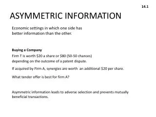
Market for Lemons • Nice simple mathematical example of how asymmetric information (AI) can force markets to unravel • Attributed to George Akeloff, Nobel Prize a few years ago • Good starting point for this analysis, although it does not deal with insuance
Problem Setup • Market for used cars • Sellers know exact quality of the cars they sell • Buyers can only identify the quality by purchasing the good • Buyer beware: cannot get your $ back if you buy a bad car
Two types of cars: high and low quality • High quality cars are worth $20,000, low are worth $2000 • Suppose that people know that in the population of used cars that ½ are high quality • Already a strong (unrealistic) assumption • One that is not likely satisfied
Buyers do not know the quality of the product until they purchase • How much are they willing to pay? • Expected value = (1/2)$20K + (1/2)$2K = $11K • People are willing to pay $11K for an automobile • Would $11K be the equilibrium price?
Who is willing to sell an automobile at $11K • High quality owner has $20K auto • Low quality owner has $2K • Only low quality owners enter the market • Suppose you are a buyer, you pay $11K for an auto and you get a lemon, what would you do?
Sell it for on the market for $11K • Eventually what will happen? • Low quality cars will drive out high quality • Equilibrium price will fall to $2000 • Only low quality cars will be sold
Some solutions? • Deals can offer money back guarantees • Does not solve the asymmetric info problem, but treats the downside risk of asy. Info • Buyers can take to a garage for an inspection • Can solve some of the asymmetric information problem
Insurance Example • All people have $50k income income • When health shock hits, all lose $20,000 • Two groups • Group one has probability of loss of 10% • Group two has probability of loss of 70% • Key assumption: people know their type • E(Income)1 = 0.9(50K) + 0.1(30K)=$48K • E(Income)2 = 0.3(50K) + 0.7(30K)=$36K
Suppose u=Y0.5 • Easy to show that • E(U)1 = .9(50K)0.5 + .1(30K)0.5 = 218.6 • E(U)2 = .3(50K)0.5 + .7(30K)0.5 = 188.3 • What are these groups willing to pay for insurance? • Insurance will leave them with the same income in both states of the world
In the good state, have income Y, pay premium (Prem), U=(Y-Prem)0.5 • In the bad state, have income Y, pay premium P, experience loss L, receive check from insurance for L • Uw/insurance = (Y-Prem)0.5
Group 1: Certain income that leaves them as well off as if they had no insurance • U = (Y-Prem)0.5 = 218.6, so Y-Prem = 218.62 = $47,771 • Group 2: same deal • U = (Y-Prem)0.5 = 188.3, so Y-Prem = 188.32 = $35,467
What are people willing to pay for insurance? Difference between expected income and income that gives same level • Group 1 • Y-prem = $50,000 – Prem = $47,771 • Prem =$2,229 • Group 2 • Can show that max premium = $14,533
Note that group 1 has $2000 in expected loss, but they are willing to pay $2229, or an addition $229 to shed risk • Group 2 has $14,000 in expected loss, they are willing to pay $14,533 or an extra $533 • Now lets look at the other side of the ledger
Suppose there is an insurance company that will provide actuarially fair insurance. • But initially they cannot determine where a client is type 1 or 2 • What is the expected loss from selling to a particular person? • E(loss) = 0.5*0.1*20K + 0.5*0.7*20K = $8K
The insurance company will offer insurance for $8000. • Note that group 1 is only willing to pay $2229 so they will decline • Note that group 2 is willing to pay $14,533 so they will accept • The only people who will accept are type II • Will the firm offer insurance at $8000?
The inability of the insurance company to determine a priori types 1 and 2 means that firm 1 will not sell a policy for $8000 • Asymmetric information has generated a situation where the high risks drive the low risk out of the insurance market • What is the solution?
Rothschild-Stiglitz • Formal example of AI/AS in insurance market • Incredibly important theoretical contribution because it defined the equilibrium contribution • Cited by Nobel committee for Stioglitz’s prize (Rothschild was screwed)
p = the probability of a bad event • d = the loss associated with the event • W=wealth in the absence of the event • EUwi = expected utility without insurance • EUwi = (1-p)U(W) + pU(W-d)
Graphically illustrate choices • Two goods: Income in good and bad state • Can transfer money from one state to the other, holding expected utility constant • Therefore, can graph indifference curves for the bad and good state of the work • EUwi = (1-p)U(W) + pU(W-d) = (1-P)U(W1) + PU(W2) • Hold EU constant, vary W1 and W2
W2(Bad) Wb EU1 W1(Good) Wa
W2(Bad) As you move NE, Expected utility increases Wc EU2 Wb EU1 W1(Good) Wa
What does slope equal? • EUw = (1-p)U(W1) + pU(W2) • dEUw = (1-p)U’(W1)dW1 + pU’(W2)dW2=0 • dW2/dW1 = -(1-p)U’(W1)/[pU’(W2)]
MRS = dW2/dW1 • How much you have to transfer from the good to the bad state to keep expected utility constant
W2(Bad) Slope of EU2 is what? MRS = dW2/dW1 What does it measure? W2 EU2 EU1 W1(Good) W1
W2(Bad) f Wd e Wb EU1 Wa W1(Good) Wc
At point F • lots of W2 and low MU of income • Little amount of W1, MU of W1 is high • Need to transfer a lot to the bad state to keep utility constant • At point E, • lots of W1 and little W2 • the amount you would need to transfer to the bad state to hold utility constant is not much: MU of good is low, MU of bad is high
Initial endowment • Original situation (without insurance) • Have W in income in the good state • W-d in income in the bad state • Can never do worse than this point • All movement will be from here
Bad a EUw/o W-d Good W
Add Insurance • EUw = expected utility with insurance • α1 pay for the insurance (premium) • α2 net return from the insurance (payment after loss minus premium) • EUw = (1-p)U(W- α1) + pU(W-d+α2)
Insurance Industry • With probability 1-p, the firm will receive α1 and with probability p they will pay α2 • π = (1-p) α1 - p α2 • With free entry π=0 • Therefore, (1-p)/p = α2/ α1 • (1-p)/p is the odds ratio • α2/ α1 = MRS of $ for coverage and $ for premium – what market says you have to trade
Fair odds line • People are endowed with initial conditions • They can move from the endowment point by purchasing insurance • The amount they have to trade income in the good state for income in the bad state is at fair odds • The slope of a line out of the endowment point is called the fair odds line • When purchasing insurance, the choice must lie along that line
Fair odds line Slope = -(1-p)/p Bad a EUw/o W-d Good W
We know that with fair insurance, people will fully insure • Income in both states will be the same • W- α1 + W-d+α2 • So d= α1+ α2 • Let W1 be income in the good state • Let W2 be income in the bad state
dEUw = (1-p)U’(W1)dW1 + pU’(W2)dW2=0 • dW2/dW1 = -(1-p)U’(W1)/[pU’(W2)] • But with fair insurance, W1=W2
U’(W1) = U’(W2) • dW2/dW1 = -(1-p)/p • Utility maximizing condition with fair insurance MRS equals ‘fair odds line’
What do we know • With fair insurance • Contract must lie along fair odds line (profits=0) • MRS = fair odds line (tangent to fair odds line) • Income in the two states will be equal • Graphically illustrate
Fair odds line Slope = -(1-p)/p Bad 450 line b W* EUw a EUw/o W-d W* Good W
Consider two types of people • High and low risk (Ph > Pl) – • Only difference is the risk they face of the bad event • Question: Given that there are 2 types of people in the market, will insurance be sold?
Define equilibrium • Two conditions • No contract can make less than 0 in E(π) • No contract can make + E(π) • Two possible equilibriums • Pooling equilibrium • Sell same policy to 2 groups • Separating equilibrium • Sell two policies
EUh = (1-ph)U(W- α1) + phU(W-d+α2) • EUl = (1-pl)U(W- α1) + plU(W-d+α2) • MRSh = (1-ph)U’(W- α1)/[phU’(W-d+α1)] • MRSl = (1-pl)U’(W- α1)/[plU’(W-d+α1)] • With pooling equilibrium, income will be the same for both people
Compare |MRSh| vs |MRSl| • Since income will be the same for both people, U’(W- α1) and U’(W-d+α1) cancel • |MRSh| vs |MRSl| • |(1-ph)/ph| vs. |(1-pl)/pl| • Since ph>pl and ph is low then can show that |MRSh| < |MRSL|
Note that |MRS#1| < |MRS#2| Bad #1 EUh Recall that |MRSH| < |MRSL| C ● MRS#1 EUL #2 MRS#2 Good
Price paid in the pooling equilibrium will a function of the distribution of H and L risks • Let λ be the fraction of high risk people • Average risk in the population is • p* = λph + (1- λ)pl • Actuarially fair policy will be based on average risk • π = (1-p*) α1 - p*α2 = 0