Download
1 / 41
410 likes | 590 Vues
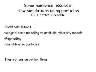
Some numerical issues in flow simulations using particles G.-H. Cottet, Grenoble. Field calculations subgrid-scale modeling vs artificial viscosity models Regridding Variable-size particles. Illustrations on vortex flows. Vorticity conservation for incompressible flows.

E N D
Some numerical issues in flow simulations using particles G.-H. Cottet, Grenoble • Field calculations • subgrid-scale modeling vs artificial viscosity models • Regridding • Variable-size particles Illustrations on vortex flows
Vorticity conservation for incompressible flows Incompressible Navier-Stokes equations in velocity-pressure formulation
Other types of particles: vorticity contours and filaments Vorticity filament: a curve that concentrates a vortex tube Circulation of vortex tube
Velocity must be computed in self-consistent way from vorticity: • Two classical approaches: • a completely grid-free approach, based on integral representation formulas • an approach using grid-based Poisson solvers • First approach uses Biot-Savart law:
When w replaced by a set of particles, velocity on each particle is expressed as • Two remarks: • Kernel is singular: need to mollify to avoid large values when particles • Approach • N-body problem: complexity in O(N2) if N=number of particles Mollification is performed by convolution with cut-off with radial symmetry and core size e -> explicit algebraic formulas High order formulas obtained by imposing that cut-off shares as many moments as possible with Dirac function Example of formula at order 4:
Complete numerical method can be rephrased as a set of coupled differential equations: Some natural conservation properties result from this formulation
O(N2) complexity can be reduce to O(NLogN) by using Fast Summation Algorithms: idea is to replace kernel by algebraic expansions: (Greengard-Rocklin, for logarithmic kernel) with precise estimates
Typical tree-code: Divide recursively into boxescontaining about the same number of particles Upward pass: form mulipole expansions, from finer to coarser level (using shifts of previously computed expansions) Downward pass: accumulate contributions of well-separated boxes, from coarser to finer level At finest level, complete with direct summation of nearby particles Still many improvements to come in 3D
Other approach for field calculations: use an underlying Eulerian grid and grid-based Poisson solvers (Particle-In-Cell/Vortex-In-Cell methods): • Project particle strength on grid points • Use a Poisson solver on that grid, and differentiate on the grid to get grid field values • Interpolate back fields on particles • Drawbacks: • against Lagrangian features of particles (and possible loss of information in grid-particle interpolations) • require far-field artificial boundary conditions • Advantage: • Cheap (for relatively simple geometries)
Tree code VIC3 direct summation VIC2 VIC1 Comparison of CPU times for velocity evaluations in 3D (Krasny tree-code vs VIC with Fishpack and 64 points interpolation formulas) VIC1: cartesiangrid with 100% particles VIC2: polar grid with 65% particles VIC3: polar grid with 25% particles
Cylindrical grid: 256x128x128 in a domain filled with 25% particles CPU time: 3mn/RK4 iteration on alpha single processor, 3hours/shedding cycle Conclusion: choice of solver depends on how localized vorticity is in the computational box needed: Flow past a sphere: grid-free calculation (Ploumehans et al.,JCP02) Flow past a cylinder: VIC calculation (C.-Poncet, JCP03) About 600,000 particles, Total cpu is 200 hours on 32 HP processors
Possible to combine both approaches (grid-free and particle-in-cell) through domain decomposition approaches: far-field by grid-free, “boundary layer” by PIC. Other issue related to velocity evaluations: time-stepping to push particles and update strengths In general RK2 or RK4 Linear stability only requires particle not to cross each other (no conventional CFL type condition): CPU savings depend on particular flow
Particle resampling schemes for diffusion Based on rewriting diffusion as an integral operator Where h satisfies moment properties:
Resulting particle scheme Here, we distinguish local values and volumes that make the particles strengths Not constrained with time-stepping, can be high order Slightly more expensive than random walk
Focus on 3D Euler equations (inviscid flows) in vorticity formulation Particle solution given by where is a mollified velocity field. weak solution to Implicit subgrid-scale models in particle methods
Mollified particles (blobs) thus satisfy This is an averaged Euler equations This means that the particle method is achieving some subgrid scale (implicit) model It thus allows for backscatter energy. Same remark applies to particle methods for compressible flows: potential increase in enstrophy (resp energy) must be compensated by diffusion term.
In 1D “optimal” form of artificial viscosity can be derived rigorously from energy principle: Equivalent equation for particles Modified ‘non energy-increasing’ equation Can be interprated as a diffusion model to correct for energy increasing part of truncation error in PM Resulting particle AV scheme
Remark: reminiscent to LES models for turbulent flows “Gradient” model Integral approximations of diffusion tensors allows to identify Positive contributions to dissipation. For incompressible flows: Where z is a cut-off function z non-increasing function of radius gives a 3d version of previous AV model
In all particle simulations, accuracy requires frequent and accurate regridding « classical » interpolation formulas
random init quiet start init quiet start init with remeshing Error curves Typical example showing importance of regridding: circular patch with high strain
1d Burger’s equation: comparison of PM (including AV and regridding) with 3rd order WENO schemes Steady shock Moving shock Black circles: PM White circles: WENO E-O White sqaures: WENO L-F
Gas dynamics for compressible isentropic viscous flows Conservation of density, momentum and energy: Comparaison of PIC method with TVD schemes for a 2D shock boundary layer interaction
Re=200, t=1 N=1000 N=500 PIC TVD (Mac-Cormack with 3rd order limiter) Tenaud-Daru
Regridding can also be used as a way to adapt particles • to the flow topology -> variable-size particles • three different approaches: • Regridding into variable-sized particles via global mappings • Regridding via local mappings • Regridding onto piecewise uniform particles
Physical space Mapped space
1) Mollified particles (for field evaluation) with blob size 2) Diffusion in mapped coordinates: Can be written in divergence form, using the fact that /
Using particle diffusion formulas for anisotropic diffusion (Degond-Mas-Gallic, 1989) we obtain
-> Remark: conservative in physical variables
Example: rebound of a dipole with exponentially stretched particle distribution (C-Koumoutsakos, JCP 00)
T=2 T=0 Coarse to fine grid fine grid Coarse grid:wrong result T=2 T=2
Variable-size particles can be used in an adaptive fashion • Two possible strategies (Bergdorf,C.,Koumoutsakos, SIAM MMS): • Adaptively build global mappings • Adaptively define zones with piecewise constant volumes • (AMR approach)
First approach: define global mappings through finite-dimensional maps: Previous strategy would require to invert the mapping. Alternative approach: move particles in the mapped space: Example: 1D convection-diffusion equation: Mapping jacobian Mapping velocity
With: Easy to derive motion equations in mapped space: And to discretize on particles
Method of adaptation relies on r-adaptive FEM: map Velcoity given by Where M monitors the regularity of the solution
Second approach: particles have piecewise constant volumes Inside each population, particles dynamics is straightforward Remeshing allows to transfer information between populations through a buffer zone:
Illustration: case of an elliptical vortex Adaptation based on vorticity gradients Fine and coarse zone in the AMR approach defined using a package designed for FD
Global mapping approach: Particle grid Vorticity contours
Measure of accuracy/cost: enstrophy profiles and number of particles compared to uniform size particles Dotted line: uniform particle distribution
Conclusion: • About AV: more to learn about specifics of PM in small-scale parametrizations • About adaptive methods: • AMR approach more “straightforward” but accuracy • strongly dependent on definition of fine and coarse grids (in progress: gas dynamics coupled with radiative transfer for inertial fusion) • Global mapping approach more subtle to implement but optimally accurate