Download
1 / 42
460 likes | 664 Vues
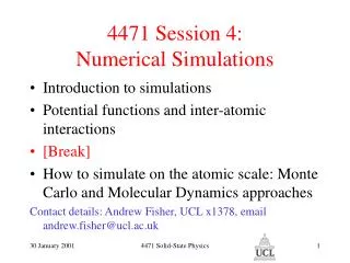
4471 Session 4: Numerical Simulations. Introduction to simulations Potential functions and inter-atomic interactions [Break] How to simulate on the atomic scale: Monte Carlo and Molecular Dynamics approaches Contact details: Andrew Fisher, UCL x1378, email andrew.fisher@ucl.ac.uk.

E N D
4471 Session 4:Numerical Simulations • Introduction to simulations • Potential functions and inter-atomic interactions • [Break] • How to simulate on the atomic scale: Monte Carlo and Molecular Dynamics approaches Contact details: Andrew Fisher, UCL x1378, email andrew.fisher@ucl.ac.uk 4471 Solid-State Physics
The idea of (atomistic)simulation • This course is about structureof materials and its relationship to properties • The simulation approach: start from atoms and the interactions between them + Interactions 4471 Solid-State Physics
The idea of (atomistic)simulation • Deduce the equilibrium structure of the system, and other properties: • Macroscopic variables (e.g. pressure, volume) • Measurable structural parameters for comparison with experiment (e.g. structure factor for a liquid, lattice vectors for a crystal) • Quantities not directly related to structure (e.g. electrical properties) + Interactions Structure Propertiese.g. S(q,), p(V,T), 4471 Solid-State Physics
Why do this? • Point is not (just) to reproduce the results of experiments • Aim to • Gain confidence to calculate quantities that cannot easily be measured • Gain understanding of relationships between physical quantities in situations too complicated to treat by analytical theory 4471 Solid-State Physics
Warnings • Simulation can be deceptively easy to do; they are not a substitute for experiment or understanding • Results are entirely dependent on • Choosing a good enough form for the interatomic interactions • Using a suitable simulation algorithm to extract the physics one is interested in • Garbage in, garbage out! 4471 Solid-State Physics
Inter-atomic interactions • Born-Oppenheimer approximation • Variational Principle and Hellman-Feynman theorem • Simple empirical potentials • First-principles routes to interatomic interactions: Hartree-Fock and Density Functional Theory • Modern approximations informed by first-principles results 4471 Solid-State Physics
The Born-Oppenheimer Approximation (1) • In a condensed-phase system the electron distributions of the atoms overlap strongly • The interatomic forces and potential energy are determined by the behaviour of the bonding electrons, which itself depends on the atomic structure • Formalise this within the Born-Oppenheimer approximation: Electron wavefunction for given nuclear positions R Full wavefunction Electron coordinates Atomic (nuclear) positions Nuclear wavefunction 4471 Solid-State Physics
The Born-Oppenheimer Approximation (2) • Nuclear wavefunction obeys the Schrödinger equation • For many purposes (including everywhere in this lecture) it’s OK to replace this nuclear Schrödinger equation by its classical approximation, so the nuclei obey Newton’s classical laws of motion 4471 Solid-State Physics
Electron-nucleus interaction Electron-electron interaction Electron K.E. Nucleus-nucleus interaction The Born-Oppenheimer Approximation (3) • The effective potential for the nuclei is determined by solving the electronic Schrödinger equation and then adding in the nuclear-nuclear repulsion: I,J label atoms with positions RI, RJ i,j label electrons with positions ri, rj 4471 Solid-State Physics
The variational principle and the Hellman-Feynman theorem (1) • In the vast majority of cases the system moves on the ground-state potential surface, for which the electronic energy is the minimum possible (subject to maintaining the normalization of the wavefunction): 4471 Solid-State Physics
Implicit dependence of E on R via the change in wavefunction as atoms move Explicit dependence of H on R The variational principle and the Hellman-Feynman theorem (2) • For a general electron state we would have to remember that the electronic energy depends on the state, as well as explicitly on the atomic positions • In order to find the force on any particular atom, we would therefore have use the chain rule to write 4471 Solid-State Physics
The variational principle and the Hellman-Feynman theorem (3) • For the ground state (or indeed any electronic eigenstate) the electronic energy is stationary with respect to variations in • We can therefore ignore the second term, to get • Force just involves calculating the electric field at the nuclear site from the charge distribution of electrons Electric field produced by electron charge distribution Only part of electronic Hamiltonian depending explicitly on atomic positions 4471 Solid-State Physics
Simple empirical potentials • Capture very simple interactions between atoms • Usually work in situations where it is easy to identify individual `atomic’ charge distributions, and these do not vary strongly as the atoms move around • We will look at three often used examples: • `Hard-sphere’ potentials • Models of rare-gas liquids and solids • Models of strongly ionic solids and liquids (point charges, shell model, and other polarizable ion models) 4471 Solid-State Physics
Hard-sphere potential V • Atoms modelled by hard spheres that never overlap: • Not a realistic model for physical systems but considerable historical interest (was among first systems simulated, exhibits entropy-driven phase freezing) and useful as a reference point for thermodynamic integration (see later) Forbidden region Allowed region r 4471 Solid-State Physics
Interactions of rare-gas atoms V • Rare-gas atoms have chemically-inert closed shells of electrons • Dominant features are • Long-range attraction via Van der Waals forces • Sort-range replulsion from overlap of electron clouds • Captured by potentials such as Lennard-Jones: R V=- R= R=21/6 4471 Solid-State Physics
- - - - - - - - + + + + + + + + Strongly ionic materials: point ion model • Interactions driven by a transfer of electron(s) from one species to another, creating positively and negatively charged ions • Point ion model: these ions interact with one another like point charges 4471 Solid-State Physics
- - - - - - - - + + + + + + + + Strongly ionic materials: point ion model (2) • Unlike Lennard-Jones potential, potential at any given site is not dominated by the nearest neighbours • Instead, must perform sum to infinity- this sum is not `absolutely convergent’ so the order of terms matters (corresponds to different terminations of the material) 4471 Solid-State Physics
Strongly ionic materials: shell model • Next level of refinement: introduce a `shell’ which can move independently of the ion core • Adjust position of `shell’ to minimise the local energy: corresponds to a dipole moment Core charge Xe - Shell charge Ye Xe+Ye=Ze (full ion charge) Atomic polarizability Local electric field 4471 Solid-State Physics
Strongly ionic materials - summary • Shell and point-ion models work best for very highly ionic solids such as alkali halides (Group I + Group VII) • For materials such as oxides there is more covalent character in the bonding Either introduce a complicated dependence of the polarizability on the environment, or treat the covalent bonding explicitly (e.g. by first-principles techniques) 4471 Solid-State Physics
- - - - - - - - - - - - - - - - + + + + + + + + + + + + + + + ‘Ab initio’ approaches • Choosing the right interatomic potential is a delicate and subtle business. • Potentials that work in one environment (e.g. a perfect crystal) may fail in another (e.g. a defective or disordered material) X 4471 Solid-State Physics
- + ‘Ab initio’ approaches - the ideal • Aim to get round this by calculating electronic energy directly from the principles of quantum mechanics • If done properly, such calculations will automatically be ‘transferable’, since they embody no information specific to a particular structure (r) Assume some V(R) Deduce Veff(R) 4471 Solid-State Physics
‘Ab initio’ approaches - the problem • Need to solve the N-particle Schrödinger equation • For one electron, might do this by expanding in terms of a complete set of basis states {}: For M basis states, there are M unknown coefficients {c} 4471 Solid-State Physics
‘Ab initio’ approaches - the problem • But for N electrons, the wavefunction has to depend on all N variables • Taking account of the Pauli exclusion principle, suitable N-electron basis functions are Slater determinants: • The number of determinants (and hence of unknown expansion coefficients) increases very rapidly - as 1-electron basis functions N-electron basis function 4471 Solid-State Physics
‘Ab initio’ approaches - the problem • Example: consider a situation with 4 outer electrons per atom (e.g. carbon or silicon) and 8 basis functions per atom (e.g. s, px, py, pz with spin up and spin down) • 8 electrons: number of coefficients needed is 12870 • 20 electrons: number of coefficients needed is 1.381011 • 40 electrons: number of coefficients needed is 1.081023 • Continues to grow exponentially with system size 4471 Solid-State Physics
The Hartree-Fock Approximation • Ideally we would like to recover a set of independent Schrödinger equations for N separate electrons (as treated in elementary solid-state physics courses!) • One way of doing this: restrict the expansion of the wavefunction to a single optimized determinant One-particle states optimized to give lowest total energy 4471 Solid-State Physics
The Hartree-Fock Approximation • This approach omits correlation between the electrons • The one-electron orbitals are determined by an effective Schrödinger-like equation: • Each individual is a one-electron function, so need only N M variational parameters (many fewer) `Exchange potential’ - purely quantum, comes from Pauli principle `Hartree potential’ - potential of classical electron charge distribution Interaction with external potential (nuclei) 4471 Solid-State Physics
The Hartree-Fock Approximation • Caution: the total electronic energy is not the sum of the Hartree-Fock eigenvalues (this would double-count the electron-electron interaction terms) • The difficulty: the exchange term is quite difficult to evaluate since it is non-local • Still have no account at all of correlation between electrons of opposite spin • Solution to (some of) these difficulties: Density Functional Theory (Hohenberg and Kohn 1964; Nobel Prize 1999) 4471 Solid-State Physics
Density Functional Theory • Energy of a system of electrons can (in principle) be written in a way that depends only on the electron charge density (r) • This is so because no two ground states for different potentials can have the same charge density • Write total energy as K.E. of noninteracting particles at this density Interaction with external potential Interaction with Hartree potential The rest! 4471 Solid-State Physics
Density Functional Theory (2) • Enables one to derive an exact set of one-electron equations • Problem: all the nasty bits (including exchange) are now swept up into the exchange-correlation energy • A simple approximation, the Local Density Approximation, is surprisingly good: approximate exchange-correlation energy per electron at each point by its value for a homogeneous electron gas of the same density 4471 Solid-State Physics
Simulation methods • Static calculations • Molecular dynamics • Monte Carlo methods 4471 Solid-State Physics
Static methods • Based on minimizing the energy as a function of the atomic configuration • Appropriate when total energy dominates fluctuations (i.e. for solids, low temperatures) • Tricky issues: • Avoiding getting `stuck’ in false energy minima • Finding efficient algorithms to cope with an energy surface that has very different slopes in different directions (e.g. a steep `valley’ with a shallow `bottom’) • Coping with long-range parts of the force • Indluing finite-temperature effects (expand potential about ground-state position, treat as collection of harmonic oscillators) 4471 Solid-State Physics
Molecular Dynamics (1) • Basic idea: simply follow Newton’s equations of motion for the atoms • Break time into discrete `steps’ t, compute forces on atoms from their positions at each timestep • Evolve positions by, for example, Verlet algorithm... • ...or the equivalent `velocity Verlet’ scheme 4471 Solid-State Physics
Molecular Dynamics (2) • Follow the `trajectory’ and use it to sample the states of the system • Assuming forces are conservative, the total energy will be conserved with time (to order (t)2 in the case of Verlet) • So, the system samples the ‘microcanonical’ (constant-energy) thermodynamic ensemble, provided that the trajectory eventually passes through all states with a given energy • Requires that there should be no conserved quantities in the dynamics apart from the total energy (ergodicity) 4471 Solid-State Physics
Molecular Dynamics (3) • Refinements exist to allow simulations at • Constant temperature (an additional variable is connected to the system which acts as a ‘heat bath’) • Constant pressure (the volume of the system is allowed to fluctuate) • Constant stress (the shape, as well as the volume, of the system is allowed to fluctuate) • Can be combined especially efficiently with ab initio density functional theory: electronic states are evolved continuously as the atoms are propagated, in order to keep the atomic forces (calculated by Hellman-Feynman) up to date 4471 Solid-State Physics
Monte Carlo Methods (1) • For a system in thermal equilibrium, know the probability P that it should occupy any given microstate r: • So in principle can find the thermodynamic average of any quantity by summing over all microstates: for example, for the energy, 4471 Solid-State Physics
Monte Carlo Methods (2) • The catch: there are usually far too many microstates to evaluate this sum explicitly • Example: suppose we have N atoms and we need to sample 10 positions of each atom to average properly. We need 10N points to perform the whole average. • The Monte Carlo method: replace the whole sum by a sample of a selected set of states 4471 Solid-State Physics
Monte Carlo sampling procedures (1) • Could in principle select states completely at random (with uniform probability) - but this would very often pick a high-energy state with negligible probability of occurrence • Instead, arrange that each state r is selected with a probability equal to its probability Pr of appearing in thermal equilibrium, so more likely states appear more often • Ideally would like the states to be drawn independently from this distribution; in practice this is very difficult because we do not know the partition function Z 4471 Solid-State Physics
Monte Carlo sampling procedures (2): Markov processes • Generate a sequence of configurations via a Markov process: at each step generate a new configuration with a probability that depends only on the current configuration, not on the history • For a stationary Markov process the transition probabilities W remain fixed with time Transition probability W(rr’) 4471 Solid-State Physics
Monte Carlo sampling procedures (3): Detailed Balance • Two important requirements for the Markov chain: • The microreversibility (or detailed balance) condition: • The accessibility condition: every configuration of the system must be accessible from every other in a finite number of steps (necessary to prevent the system becoming `trapped’ and never sampling parts of configuration space) 4471 Solid-State Physics
Monte Carlo sampling procedures (4) • The Metropolis algorithm (Metropolis et al 1953): choose a new configuration from the old one by making some trial change in a way that treats the old and new configurations symmetrically (e.g. move one atom randomly within a sphere of selected radius) Accept r’ Trial r r r’ Reject 4471 Solid-State Physics
Monte Carlo sampling procedures (5) • Accept trial configuration as new configuration with probability Accept r’ Trial r r r’ Reject 4471 Solid-State Physics
Making use of Monte Carlo • To think about: given a sequence of configurations generated by the Metropolis algorithm, how would you find • The mean energy of the system? • An estimate for the statistical error in the energy? • The pair correlation function? • The heat capacity? • The free energy? 4471 Solid-State Physics