Download
1 / 112
1.13k likes | 1.28k Vues
Information Theory, Statistical Measures and Bioinformatics approaches to gene expression. Friday’s Class. Sei Hyung Lee will make a presentation on his dissertation proposal at 1pm in this room Vector Support Clustering So I will discuss Clustering and other topics. Information Theory.

E N D
Information Theory, Statistical Measures and Bioinformatics approaches to gene expression
Friday’s Class • Sei Hyung Lee will make a presentation on his dissertation proposal at 1pm in this room • Vector Support Clustering • So I will discuss Clustering and other topics
Information Theory • Given a probability distribution, Pi, for the letters in an independent and identically distributed (i.i.d.) message, the probability of seeing a particular sequence of letters i, j, k, ..., n is simply Pi Pj Pk···Pn or elog Pi + log Pj + log Pk+ ··· + log Pn
Information Theory 2 • The information or surprise of an answer to a question (a message) is inversely proportional to its probability – the smaller the probability, the more surprise or information • Ask a child “Do you like ice cream?” • If the answer is yes, you’re not surprised and the information conveyed is little • If the answer is no, you are surprised – more information has been given with this lower probability answer
Information Theory 3 Information H associated with probability p is H(p) = log2 (1/p) 1/p is the information or surprise and log2 (1/p) = # of bits required
Information Theory 4 Log-probabilities and their sums represent measures of information. Conversely, information can be thought of as log-probabilities (with the negative sign to make the information increase with increasing values) H(p) = log2 (1/p) = - log2 p
Information Theory 5 If we have an i.i.d. with 6 values (a die), or 4 (A, C, T, G) or n values (the distribution is flat) then the probability of any particular symbol is 1/n and the information in any such symbol is then log2 n and this value is also the average If the symbols are not equally probable (not i.d.) we need to weigh the information of each symbol by its probability of occurring. This is Claude Shannon’s Entropy H = Σ pi log2 (1/pi) = - Σ pi log2 pi
Information Theory 6 If we have a coin, assuming h and t have equal probabilities. H = - ( (1/2)log2 (1/2) + (1/2)log2 (1/2) ) = - ( (1/2)(-1) + (1/2)(-1) ) = - ( -1) = 1 bit If the coin comes up heads ¾ of the time then the entropy should decrease (we’re more certain of the outcome and there’s less surprise) H = - ( (3/4)log2 (3/4) + (1/4)log2 (1/4) ) = - ( (0.75)(-0.415) + (0.25)(-2) ) = - ( -0.81) = 0.81 bits
Information Theory 7 A random DNA source has an entropy of H = - ( (1/4)log2 (1/4) + (1/4)log2 (1/4) + (1/4)log2 (1/4) + (1/4)log2 (1/4) ) = - ( (1/4)(-2) + (1/4)(-2) + (1/4)(-2) + (1/4)(-2)) = - ( -2) = 2 bits A DNA source that emits 45% A and T and 5% G and C has an entropy of H = - ( 2*(0.45)log2 (0.45) + 2*(0.05)log2 (0.05)) = - ( (0.90)(-1.15) + (0.10)(-4.32) ) = - ( - 1.035 – 0.432) = 1.467 bits
Natural Logs • Using natural logarithms, the information is expressed in units of nats (a contraction of Natural digits). Bits and nats are easily convertible as follows nats = bits · ln (2) ln 2 or log 2 ≈ 0.693 1/ln 2 ≈ 1.44 • Generalizing, for a given base of the logarithm b log x = log b · logb x • Using logarithms to arbitrary bases, information can be expressed in arbitrary units, not just bits and nats, such that -logbP = -k log P , where 1/k=log bSo k is often ignored
Shannon’s Entropy • Shannon's entropy, H = Σ pi log2 (1/pi) = - Σ pi log2 pi , is the expected (weighted arithmetic mean) value of log Picomputed over all letters in the alphabet, using weights that are simply the probabilities of the letters themselves, the Pis • The information, H, is expressed in units per letter • Shannon's entropy allows us to compute the expected description length of a message, given an a priori assumption (or knowledge) that the letters in the message will appear with frequencies Pi • If a message is 200 letters in length, 200H is the expected description length for that message • Furthermore, the theory tells us there is no shorter encoding for the message than 200H, if the symbols do indeed appear at the prescribed frequencies • Shannon's entropy thus informs us of the minimum description length, or MDL, for a message
Shannon Entropy A DNA source that emits 45% A and T and 5% G and C has an entropy of H = - ( 2*(0.45)log2 (0.45) + 2*(0.05)log2 (0.05)) = - ( (0.90)(-1.15) + (0.10)(-4.32) ) = - ( - 1.035 – 0.432) = 1.467 bits
Huffman Entropy (or Encoding) If we build a binary Huffman code (tree) for the same DNA 1 bit would be required to code for G 2 bits to code for T (or vice versa) 3 bits each to code for A and C The "Huffman entropy" in this case is 1*0.45 + 2*0.45 + 3*0.05 + 3*0.05= 1.65 bits per letter -- which is not quite as efficient as the previous Shannon code
Length of Message • The description length of a message when using a Huffman code is expected to be about equal to the Shannon or arithmetic code length • Thus, a Huffman-encoded 200 letter sequence will average about 200H bits in length • For some letters in the alphabet, the Huffman code may be more or less efficient in its use of bits than the Shannon code (and vice versa), but the expected behavior averaged over all letters in the alphabet is the same for both (within one bit)
Relative Entropy • Relative entropy, H, is a measure of the expected coding inefficiency per letter, when describing a message with an assumed letter distribution P, when the true distribution is Q. • If a binary Huffman code is used to describe the message, the relative entropy concerns the inefficiency of using a Huffman code built for the wrong distribution • Whereas Shannon's entropy is the expected log-likelihood for a single distribution, relative entropy is the expected logarithm of the likelihood ratio (log-likelihood ratio or LLR) between two distributions. H(Q || P) = Σ Qi log2 (Qi /Pi)
The Odds Ratio • The odds ratioQi / Pi is the relative odds that letter i was chosen from the distribution Q versus P • In computing the relative entropy, the log-odds ratios are weighted by Qi • Thus the weighted average is relative to the letter frequencies expected for a message generated with Q H(Q || P) = Σ Qi log2 (Qi /Pi)
Interpreting the Log-Odds Ratio • The numerical sign of individual LLRs log(Qi / Pi) LLR > 0 => i was more likely chosen using Q than P LLR = 0 => i was as likely selected using Q as it was using P LLR < 0 => i was more likely chosen using P than Q • Relative entropy is sometimes called the Kullback Leibler distance between the distributions P and Q H(P || Q) ≥ 0 H(P || Q) = 0 iff P = Q H(P || Q) is generally ≠ to H(Q || P)
The Role of Relative Entropy • Given a scoring matrix (or scoring vector, in this one-dimensional case) and a model sequence generated i.i.d. according to some background distribution, P, we can write a program that finds the maximal scoring segment (MSS) within the sequence (global alignment scoring) • Here the complete, full-length sequence represents one message, while the MSS reported by our program constitutes another • For example, we could create a hydrophobicity scoring matrix that assigns increasingly positive scores to more hydrophobic amino acids, zero score to amphipathic residues, and increasingly negative scores to more hydrophilic residues. (Karlin and Altschul (1990) provide other examples of scoring systems, as well).
The Role of Relative Entropy • By searching for the MSS - the "most hydrophobic" segment in this case - we select for a portion of the sequence whose letters exhibit a different, hydrophobic distribution than the random background • By convention, the distribution of letters in the MSS is called the target distribution and is signified here by Q. (Note: some texts may signify the background distribution as Q and the target distribution as P).
The Role of Relative Entropy 2 • If the letters in the MSS are described using an optimal Shannon code for the background distribution, we expect a longer description than if a code optimized for the target distribution was used instead • These extra bits -- the extra description length -- tell us the relative odds that the MSS arose by chance from the background distribution rather than the target • Why would we consider a target distribution, Q, when our original sequence was generated from the background distribution, P? • Target frequencies represent the underlying evolutionary model • The biology tells us that • The target frequencies are indeed special • The background and target frequencies are formally related to one another by the scoring system (the scoring matrices don’t actually contain the target frequencies but they are implicit in the score) • The odds of chance occurrence of the MSS are related to its score
BLAST Scoring Database similarity searches typically yield high-scoring pairwise sequence alignments such as the following Score = 67 (28.6 bits), Expect = 69., P = 1.0 Identities = 13/33 (39%), Positives = 23/33 (69%) Query: 164 ESLKISQAVHGAFMELSEDGIEMAGSTGVIEDI 196 E+L + Q+ G+ ELSED ++ G +GV+E++ Subjct: 381 ETLTLRQSSFGSKCELSEDFLKKVGKSGVVENL 413 +++-+-++--++--+++++-++- + +++++++ Scores: 514121512161315445632110601643512 • The total score for an alignment (67 in the above case) is simply the sum of pairwise scores • The individual pairwise scores are listed beneath the alignment above (+5 on the left through +2 on the right)
Scoring Statistics • Note that some pairs of letters may yield the same score • For example, in the BLOSUM62 matrix used to find the previous alignment, S(S,T) = S(A,S) = S(E,K) = S(T,S) = S(D,N) = +1 • While alignments are usually reported without the individual pairwise scores shown, the statistics of alignment scores depend implicitly on the probabilities of occurrence of the scores, not the letters. • Dependency on the letter frequencies is factored out by the scoring matrix. • We see then that the "message" obtained from a similarity search consists of a sequence of pairwise scores indicated by the high-scoring alignment
Karlin-Altschul Statistics 1 If we search two sequences X and Y using a scoring matrix Sij to identify the maximal-scoring segment pair (MSP), and if the following conditions hold • the two sequences are i.i.d. and have respective background distributions PX and PY (which may be the same), • the two sequences are effectively "long" or infinite and not too dissimilar in length, • the expected pairwise score Σ PX(i) PY(j) Sij is negative, • a positive score is possible, i.e., PX(i)PY(j)Sij > 0 for some letters i and j, then
Karlin-Altschul Statistics 2 • The scores in the scoring matrix are implicitly log-odds scores of the form Sij = log(Qij / (PX(i)PY(j))) / l where Qij is the limiting target distribution of the letter pairs (i,j) in the MSP and l is the unique positive-valued solution to the equation ΣPX(i) PY(j) e l Sij = 1 • The expected frequency of chance occurrence of an MSP with score S or greater is E = K mn e-lS where m and n are the lengths of the two sequences, mn is the size of the search space, and K is a measure of the relative independence of the points in this space in the context of accumulating the MSP score • While the complete sequences X and Y must be i.i.d., the letter pairs comprising the MSP do exhibit an interdependency
Karlin-Altschul Statistics 3 • Since gaps are disallowed in the MSP, a pairwise sequence comparison for the MSP is analogous to a linear search for the MSS along the diagonals of a 2-d search space. The sum total length of all the diagonals searched is just mn • Another way to express the pairwise scores is: Sij = logb(Qij / (PX(i)PY(j))) Where the log is to some base b and l = loge b, and is often called the scale of the scoring matrix
Karlin-Altschul Statistics 4 • The MSP score is the sum of the scores Sij for the aligned pairs of letters in the MSP (the sum of log-odds ratios) • The MSP score is then the logb of the odds that an MSP with its score occurs by chance at any given starting location within the random background -- not considering yet how large an area, or how many starting locations, were actually examined in finding the MSP • Considering the size of the examined area alone, the expected description length of the MSP (measured in information) is log(K m n) • The relative entropy, H, has units of information per length (or letter pair), the expected length of the MSP (measured in letter pairs) is E(L) = log(K m n) / H where H is the relative entropy of the target and background frequencies H= Σ Qij log(Qij / (PX(i) PY(j))) where PX(i) PY(j) is the product frequency expected for letter i paired with j in the background search space; and Qij is the frequency at which we expect to observe i paired with j in the MSP
Karlin-Altschul Statistics 5 • By definition, the MSP has the highest observed score. Since this score is expected to occur just once, the (expected) MSP score has an (expected) frequency of occurrence, E, of 1 • The appearance of MSPs can be modeled as a Poisson process with characteristic parameter E, as it is possible for multiple, independent segments of the background sequences to achieve the same high score • The Poisson "events" are the individual MSPs having the same score S or greater • The probability of one or more MSPs having score S or greater is simply one minus the probability that no MSPs appear having score S or greater P = 1 - e-E • Note that in the limit as E approaches 0, P = E; and for values of E or P less than about 0.05, E and P are practically speaking equal
Karlin-Altschul Statistics 6 • For convenience in comparing scores from different database searches, which may have been performed with different score matrices and/or different background distributions, we can compute the normalized or adjusted score S' = lS - log K • Expressing the "Karlin-Altschul equation" as a function of the adjusted score, we obtain E = mn e-S' • Note how the search-dependent values for l and K have been factored out of the equation by using adjusted scores • We can therefore assess the relative significance of two alignments found under different conditions, merely by comparing their adjusted scores. To assess their absolute statistical significance, we need only know the size of the search space, mn.
Karlin-Altschul Statistics 7 • Biological sequences have finite length, as do the MSPs found between them • MSPs will tend not to appear near the outer (lower and right) edges of the search space • The chance of achieving the highest score of all are reduced in that region because the end of one or both sequences may be reached before a higher score is obtained than might be found elsewhere • Effectively, the search space is reduced by the expected length, E(l), for the MSP • We can therefore modify the Karlin-Altschul equation to use effective lengths for the sequences compared. m' = m - E(l) and n' = n - E(l) E' = K m' n' e-lS • Since m' is less than m and n' is less than n, the edge-corrected E' is less than E, indicating greater statistical significance.
Karlin-Altschul Statistics 8 • A raw MSP or alignment score is meaningless (uninformative) unless we know the associated value of the scaling parameter l, to a lesser extent K, and the size of the search space • Even if the name of the scoring matrix someone used has been told to us (e.g., BLOSUM62), it might be that the matrix they used was scaled differently from the version of the matrix we normally use • For instance, a given database search could be performed twice, with the second search using the same scoring matrix as the first's but with all scores multiplied by 100 • While the first search's scores will be 100-fold lower, the alignments produced by the two searches will be the same and their significance should rightfully be expected to be the same • This is a consequence of the scaling parameter l being 100-fold lower for the second search, so that the product lS is identical for both searches • If we did not know two different scoring matrices had been used and hadn't learned the lessons of Karlin-Altschul statistics, we might have been tempted to say that the higher scores from the second search are more significant (at the same time, we might have wondered: if the scores are so different, why are the alignments identical?!)
Karlin-Altschul Statistics 9 • Karlin-Altschul statistics suggest we should be careful about drawing conclusions from raw alignment scores • When someone says they used the "BLOSUM62" matrix to obtain a high score, it is possible their matrix values were scaled differently than the BLOSUM62 matrix we have come to know • Generally in our work with different programs, and in communications with other people, we may find "BLOSUM62" refers to the exact same matrix, but this doesn't happen automatically; it only happens through efforts to standardize and avoid confusion • Miscommunication still occasionally happens, and people do sometimes experiment with matrix values and scaling factors, so consider yourself forewarned! • Hopefully you see how the potential for this pitfall further motivates the use of adjusted or normalized scores, as well as P-values and E-values, instead of raw scores
Karlin-Altschul Statistics 10 • Statistical interpretations of results often involves weighing a null model against an alternative model • In the case of sequence comparisons and the use of Karlin-Altschul statistics, the two models being weighed are the frequencies with which letters are expected to be paired in unselected, random alignments from the background versus the target frequencies of their pairing in the MSP • Karlin and Altschul tell us when we search for the MSP we are implicitly selecting for alignments with a specific target distribution, Q, defined for seeing letter i paired with letter j, where Qij = PX(i) PY(j) elSij
Karlin-Altschul Statistics 11 • We can interpret a probability (or P-value) reported by BLASTP as being a function of the odds that the MSP was sampled from the background distribution versus being sampled from the target distribution • In each case, one considers the MSP to have been created by a random, i.i.d. process • The only question is which of the two distributions was most likely used to generate the MSP score: the background frequencies or the target frequencies?
Karlin-Altschul Statistics 12 • If the odds of being sampled from the background are low (i.e., much less than 1), then they are approximately equal to the P-value of the MSP having been created from the background distribution. Low P-values do not necessarily mean the score is biologically significant, only that the MSP was more likely to have been generated from the target distribution, which presumably was chosen on the basis of some interesting biological phenomena (such as multiple alignments of families of protein sequences) • Further interpretations, such as the biological significance of an MSP score, are not formally covered by the theory (and are often made with a rosy view of the situation) • Even if (biological) sequences are not random according to the conditions required for proper application of Karlin-Altschul statistics, we can still search for high-scoring alignments • It may just happen that the results still provide some biological insight, but their statistical significance can not be believed. Even so, if the scoring system and search algorithm are not carefully chosen, the results may be uninformative or irrelevant -- and the software provides no warning.
Gene expression is regulated in several basic ways • • by region (e.g. brain versus kidney) • • in development (e.g. fetal versus adult tissue) • • in dynamicresponse to environmental signals • (e.g. immediate-early response genes) • in disease states • by gene activity Page 157
Organism Gene expression changes measured... virus bacteria fungi invertebrates rodents human In response to stimuli Cell types In virus, bacteria, and/or host In mutant or wildtype cells Disease Development Page 158
DNA RNA protein phenotype cDNA Page 159
protein protein DNA RNA DNA RNA cDNA cDNA UniGene SAGE microarray Page 159
DNA RNA protein phenotype cDNA [1] Transcription [2] RNA processing (splicing) [3] RNA export [4] RNA surveillance Page 160
5’ 3’ exon 1 intron exon 2 intron exon 3 3’ 5’ transcription 5’ 3’ RNA splicing (remove introns) 3’ 5’ polyadenylation 5’ AAAAA 3’ Export to cytoplasm Page 161
Analysis of gene expression in cDNA libraries • A fundamental approach to studying gene expression • is through cDNA libraries. • Isolate RNA (always from a specific • organism, region, and time point) • Convert RNA to complementary DNA • Subclone into a vector • Sequence the cDNA inserts. • These are expressed sequence tags • (ESTs) insert vector Page 162-163
UniGene: unique genes via ESTs • • Find UniGene at NCBI: • www.ncbi.nlm.nih.gov/UniGene • UniGene clusters contain many ESTs • • UniGene data come from many cDNA libraries. • Thus, when you look up a gene in UniGene • you get information on its abundance • and its regional distribution. Page 164
Cluster sizes in UniGene This is a gene with 1 EST associated; the cluster size is 1 Page 164
Cluster sizes in UniGene This is a gene with 10 ESTs associated; the cluster size is 10 Page 164
Cluster sizes in UniGene Cluster size Number of clusters 1 34,000 2 14,000 3-4 15,000 5-8 10,000 9-16 6,000 17-32 4,000 500-1000 500 2000-4000 50 8000-16,000 3 >16,000 1 Page 164