Various Regularization Methods in Computer Vision
Various Regularization Methods in Computer Vision. Min- Gyu Park Computer Vision Lab. School of Information and Communications GIST. Vision Problems (intro). Such as stereo matching, optical flow estimation, de-noising, segmentation, are typically ill-posed problems .

Various Regularization Methods in Computer Vision
E N D
Presentation Transcript
Various Regularization Methods in Computer Vision Min-Gyu Park Computer Vision Lab. School of Information and Communications GIST
Vision Problems (intro) • Such as stereo matching, optical flow estimation, de-noising, segmentation, are typically ill-posed problems. • Because these are inverse problems. • Properties of well-posed problems. • Existence: a solution exists. • Uniqueness: the solution is unique. • Stability: the solution continuously depends on the input data.
Vision Problems (intro) • Vision problems are difficult to compute the solution directly. • Then, how to find a meaningful solution to such a hard problem? • Impose the prior knowledge to the solution. • Which means we constrict the space of possible solutions to physically meaningful ones.
Vision Problems (intro) • This seminar is about imposing our prior knowledge to the solution or to the scene. • There are various kinds of approaches, • Quadratic regularization, • Total variation, • Piecewise smooth models, • Stochastic approaches, • With either L1 or L2 data fidelity terms. • We will study about the properties of different priors.
Bayesian Inference & Probabilistic Modeling • We will see the simple de-noising problem. • f is a noisy input image, u is the noise-free (de-noised) image, and n is Gaussian noise. • Our objective is finding the posterior distribution, • Where the posterior distribution can be directly estimated or can be estimated as,
Bayesian Inference & Probabilistic Modeling • Probabilistic modeling • Depending on how we model p(u), the solution will be significantly different. Prior term Likelihood term (data fidelity term) Evidence(does not depend on u)
De-noising Problem • Critical issue. • How to smooth the input image while preserving some important features such as image edge. Input (noisy) image De-noised image via L1 regularization term
De-noising Problem • Formulation. Quadratic smoothness of a first order derivatives. First order: flat surface Second order: quadratic surface
De-noising Problem • By combining both likelihood and prior terms, • Thus, maximization of p(f|u)p(u) is equivalent to minimize the free energy of Gibbs distribution. Is the exactly Gibbs function!!!
How to minimize the energy function? • Directly solve the Euler-Lagrange equations. • Because the solution space is convex!(having a globally unique solution)
The Result of a Quadratic Regularizer Noise are removed (smoothed), but edges are also blurred. Input (noisy) image The result is not satisfactory….
Why? • Due to bias against discontinuities. intensity 5 4 3 2 1 0 Discontinuity are penalized more!!! 1 2 3 4 5 6 whereas L1 norm(total variation)treats both as same.
Pros & Cons • If there is no discontinuity in the result such as depth map, surface, and noise-free image, quadratic regularizer will be a good solution. • L2 regulaizer is biased against discontinuities. • Easy to solve! Descent gradient will find the solution. • Quadratic problems has a unique global solution. • Meaning it is a well-posed problem. • But, we cannot guarantee the solution is truly correct.
Introduction to Total Variation • If we use L1-norm for the smoothness prior, • Furthermore, if we assume the variance is 1 then,
Introduction to Total Variation • Then, the free energy is defined as total variation of a function u. Definition of total variation: u(x) s.t. the summation should be a finite value (TV(f) < ). Those functions have bounded variation(BV). 0 x
Characteristics of Total Variation • Advantages: • No bias against discontinuities. • Contrast invariant without explicitly modeling the light condition. • Robust under impulse noise. • Disadvantages: • Objective functions are non-convex. • Lie between convex and non-convex problems.
How to solve it? • With L1, L2 data terms, wecan use • Variational methods • Explicit Time Marching • Linearization of Euler-Lagrangian • Nonlinear Primal-dual method • Nonlinear multi-grid method • Graph cuts • Convex optimization (first order scheme) • Second order cone programming • To solve original non-convex problems.
Variational Methods • Definition. • Informally speaking, they are based on solving Euler-Lagrange equations. • Problem Definition (constrained problem). The first total variation based approach in computer vision, named after Rudin, Osher and Fatemi, shortly as ROF model (1992).
Variational Methods • Unconstrained (Lagrangian) model • Can be solved by explicit time matching scheme as,
Variational Methods • What happens if we change the data fidelity term to L1 norm as, • More difficult to solve (non-convex), but robust against outliers such as occlusion. This formulation is called as TV-L1 framework.
Variational Methods • Comparison among variational methods in terms of explicit time marching scheme. L2-L2 TV-L2 TV-L1 Where the degeneracy comes from.
Variational Methods • In L2-L2 case, where
Duality-based Approach • Why do we use duality instead of the primal problem? • The function becomes continuously differentiable. • Not always, but in case of total variation. • For example, we use below property to introduce a dual variable p,
Duality-based Approach • Deeper understandings of duality in variational methods will be given in the next seminar.
Applying to Other Problems • Optical flow (Horn and Schunck – L2-L2) • Stereo matching (TV-L1) • Segmentation (TV-L2)