Image Enhancement by Regularization Methods
Image Enhancement by Regularization Methods. Andrey S. Krylov , Andrey V. Nasonov , Alexey S. Lukin. Moscow State University Faculty of Computational Mathematics and Cybernetics Laboratory of Mathematical Methods of Image Processing. Introduction.

Image Enhancement by Regularization Methods
E N D
Presentation Transcript
Image Enhancement by Regularization Methods Andrey S. Krylov, Andrey V. Nasonov, Alexey S. Lukin Moscow State University Faculty of Computational Mathematics and Cybernetics Laboratory of Mathematical Methods of Image Processing
Introduction Many image processing problems are posed as ill-posed inverse problems. To solve these problems numerically one must introduce some additional information about the solution, such as an assumption on the smoothness or a bound on the norm. This process was theoretically proven by Russian mathematician Andrey N. Tikhonov and it is known as regularization.
Outline • Regularization methods • Applications • Resampling (interpolation) • Deringing (Gibbs effect reduction) • Super-resolution
Ill-posed Problems Formally, a problem of mathematical physics is called well-posed or well-posed in the sense of Hadamard if it fulfills the following conditions: 1. For all admissible data, a solution exists. 2. For all admissible data, the solution is unique. 3. The solution depends continuously on data.
Ill-posed Problems • Many problems can be posed as problems of solution of an equation • A is a linear continuous operator, Z and U are Hilbert spaces • The problem is ill-posed and the corresponding matrix for operator А in discrete form is ill-conditioned
Point Spread Function (PSF) PSF = Assume: Point light source
Convolution Model Generation rule:B= KL + N Notations • L: original image • K: the blur kernel (PSF) • N: sensor noise (white) • B: input blurred image +
Deblur using Convolution Theorem Convolution Theorem:
Deblur using Convolution Theorem Recovered Blurred Image PSF
Deconvolution is unstable Noisy case
Variational regularization methods • Tikhonov methods • The Residual method (Philips) • The Quasi-solution method (Ivanov)
Variational regularization methods • Regularization method is determined by: A) Choice of solution space and of stabilizer B) Choice of C) Method of minimization • A and B determine additional information on problem solution we want to use for solution of ill-posed problem to achieve stability
Outline • Regularization methods • Applications • Resampling (interpolation) • Deringing (Gibbs effect reduction) • Super-resolution
Resampling:Introduction • Interpolation is also referred to as resampling, resizing or scaling of digital images • Methods: • Linear non-adaptive (bilinear, bicubic, Lanczos interpolation) • Non-linear edge-adaptive (triangulation, gradient methods, NEDI) • Regularization method is used to construct a non-linear edge-adaptive algorithm
bilinear interpolation non-linear method Resampling:Linear and non-linear method
Resampling:Inverse problem • Consider the problem of resampling as • Problem: operator A is not invertible z is unknown high-resolution image, u is known low-resolution image, A is the downsampling operator which consists of filtering H and decimation D
Resampling:Regularization • We use Tikhonov-based regularization methodwhere
Resampling:Regularization • Choices of regularizing term (stabilizer) • Total Variation • Bilateral TV and are shift operators along x and y axes by s and t pixels respectively, p = 1, γ = 0.8
Resampling:Regularization • Minimization problem • Subgradient method
Resampling:Results • Linear method • Regularization-basedmethod • Gibbs phenomenon
Image Enhancement by Regularization Methods • Introduction to regularization • Applications • Resampling (interpolation) • Deringing (Gibbs effect reduction) • Super-resolution
Total Variation Approach for Deringing • Gibbs effect is related to Total Variation High TV, very notable Gibbs effect (ringing) Low TV
Total Variation Regularization methods • Tikhonov’sapproach • Rudin, Osher, Fatemi method • Ivanov’s quasi-solution method
Global and Local Deringing • Two approaches for Deringing • Global deringing • Minimizes TV for entire image • In this case, we use Tikhonov regularization method • No ways to estimate regularization parameter, details outside edges may be lost • Local deringing • Used if we have information on TV for small rectangular areas • In this case, we use Ivanov’s quasi-solution method for small overlapping blocks
Deringing after interpolation • Deringing after interpolation • We know information on TV for blocks of initial image to be resampled • We suggest that TV does not change after image interpolation • Thus we have real algorithm to find regularization parameter for deringing after image resampling task
Minimization • Tikhonov regularization method • Subgradient method • Quasi-solution method • 1D Conditional gradient method (there is no effective 2D implementation) • In 2D case, we divide an image into a set of rows and process these rows by 1D method, next we do the same with columns and finally we average these results
Minimization • Conditional gradient method • Conditional gradient method is used to minimize a convex functional on a convex compact set. The key idea of this method is that step directions are chosen among the vertices of the set of constraints, so we do not fall outside this set during minimization process • Conditional gradient method is effective only for small images, so it is used for local deringing only
Resampling + Deringing:PSNR Results A set of 100 nature and architecture images with 400x300 resolution (11x11 blocks, 1813 per image) was used to test the methods. We downsampled the images by 2x2 using Gauss blur with radius 0.7 and then upsampled them by our regularization algorithm. Next we applied deringing methods and compared the results with initial images.
regularization-basedinterpolation application of quasi-solution method Resampling + Deringing:Results
Resampling + Deringing:Results Regularization-based interpolation +quasi-solution deringing method Source image, upsampled by box filter Linear interpolation Regularization-based method
Image Enhancement by Regularization Methods • Introduction to regularization • Applications • Resampling (interpolation) • Deringing (Gibbs effect reduction) • Super-resolution
Super-Resolution:Introduction • The problem of super-resolution is to recover a high-resolution image from a set of several degraded low-resolution images • Super-resolution methods • Learning-based – single image super-resolution, learning database (matching between low- and high-resolution images) • Reconstruction-based – use only a set of low-resolution images to construct high-resolution image
Super-Resolution:Inverse Problem • The problem of super-resolution is posed as error minimization problem • z – reconstructed high-resolution image • vk – k-th low-resolution input image • Ak – downsampling operator, it includes motion information
Super-Resolution:Downsampling operator • Ak – downsampling operator • Hcam – camera lens blur (modeled by Gauss filter) • Hatm – atmosphere turbulence effect (neglected) • n – noise (ignored) • Fk – warping operator – motion deformation
Super-Resolution:Warping operator • Warping operator Fk
Super-Resolution:Regularization • The problem is ill-posed, and we use Tikhonov regularization approach (same as in resampling) where , • Minimization by subgradient method
Super-Resolution:Results Source images Pixel replication Linear method Non-linear method Super-resolution Face super-resolution for the factor of 4 and 10 input images
The reconstruction of an image from a sequence Super-Resolution:Results linearly interpolated single frame examples of input frames (of total 14) super-resolution result
Super-Resolution for Video current frame Super-Resolution For every frame, we take current frame, 3 previous and 3 next frames. Then we process it by super-resolution.
Super-Resolution:Results for Video Nearest neighbor interpolation Super-Resolution Super-Resolution for video for a factor of 4
Super-Resolution:Results for Video Bilinear interpolation Super-Resolution Super-Resolution for video for a factor of 4
Super-Resolution:Results for Video Bicubic interpolation Super-Resolution Super-Resolution for video for a factor of 4
Conclusion • Increasing CPU and GPU power makes regularization methods more and more important in image processing • Regularization is a very powerful tool but each specific image processing problem needs its own regularization method
http://imaging.cs.msu.ru/ Thank you!