Download
1 / 60
610 likes | 815 Vues
Image Display & Enhancement. Lecture 2 Prepared by R. Lathrop 10/99 updated 1/03 Readings: ERDAS Field Guide 5th ed Chap 4; Ch 5:137-153; App A Math Topics: 459-469. Where in the World?. http://phillips.blogs.com/photos/uncategorized/124_burning_man.jpg. Learning objectives.

E N D
Image Display & Enhancement Lecture 2 Prepared by R. Lathrop 10/99 updated 1/03 Readings: ERDAS Field Guide 5th ed Chap 4; Ch 5:137-153; App A Math Topics: 459-469
Where in the World? http://phillips.blogs.com/photos/uncategorized/124_burning_man.jpg
Learning objectives • Remote sensing science concepts • Role of additive color process in computer display • Spectral enhancement through image stretching • Image fusion • Image segmentation • Math Concepts • Summarizing image data sets • Measures of central location & dispersion • Skills • Calculating disk space of digital image • Image spectral enhancement: LUT table and stretching methods • Image fusion and basic segmentation
Analog-to-digital conversion process A-to-D conversion transforms continuous analog signal to discrete numerical (digital) representation by sampling that signal at a specified frequency Continuous analog signal Discrete sampled value Radiance, L dt Adapted from Lillesand & Kiefer
Digital Images • Measurement Vector of a pixel - is the set of data file values for one pixel in all n bands • Digital Number (DN) or Brightness Value (BV) - the tonal gray scale expressed as a number, typically 8-bit number (0-255) • Dimensionality - the number of data layers (bands)
Digital Image Band 1 Multiple spatially co-registered bands, can be displayed singly in B&W or in color composite 255 Band 2 Band 3 0 8 bit DN
Image Notation Columns = j = 5 • i = row (or line) in the image • j = column • k, l = bands of imagery • Bvijk = BV in row i, column j of band k • n = total # of pixels in an array Rows = i = 4
Calculating disk space [ ( (x * y * b) * n) ] x 1.4 = output file size in bytes where: y = rows x = columns b = number of bytes per pixel per band n = number of bands 1.4 adds 30% for pyramid layers and 10% for other info. e.g. (4*5*1)*4*1.4=896 bytes 4 bit data: b=0.5 8-bit data: b=1; 16 bit-data: b=2; 32-bit data: b=4
Digital Image Storage Formats • Band sequential (BSQ) - each band contained in a separate file • Band interleaved by line (BIL) - each record in the file contains a scan line (row) of data for one band, with successive bands recorded as successive lines • Band Interleaved by Pixel (BIP)
Summarizing data distributions • Frequency distributions - method of describing or summarizing large volumes of data by grouping them into a limited number of classes or categories • Histograms - graphical representation of a frequency distribution in the form of a bar chart
# of pixels 0 255 Digital Number Summarizing Data Distributions: Histograms Histograms
Measures of Central Location • Mean - simple arithmetic average, the sum of all observations divided by the number of observations • Median - the middle number in a data set, midway in the frequency distribution • Mode - the value that occurs with the greatest frequency, the peak in a histogram
Measures of Central Location Mode Median # of pixels Mean 0 255 Digital Number
Measures of Dispersion • Range - the difference between the largest and smallest value • Variance - the average of the squared deviations between the data values and the mean • Standard Deviation - the square root of the variance, in the units of data measurement
# of pixels Min = 60 255 0 Max = 200 Digital Number Measures of Dispersion: Range Example: Range = (max - min) = 200 - 60 = 140
Covariance & Correlation Matrices • Provide a useful summary of data relationships • High variance suggests a higher information content for that band • High correlation suggests a substantial amount of redundancy • Low correlation suggests that each band provides information not found in the other
Covariance Matrix Diagonals represent band variances. Example, variance for Band 3 = 273.1Off-diagonals represent covariances. Example, covariance of Band 1 and 4 = -35.3; same as covariance of Band 4 and 1. Negative covariance: as one band increases, the other decreases. Covariance matrix 1 2 3 4 5 6 7 1 232.3 139.1 237.2 -35.3 191.9 42.0 182.6 2 139.1 89.9 153.4 -4.6 142.1 24.1 122.0 3 237.2 153.4 273.1 -26.9 249.1 46.4 219.4 4 -35.3 -4.6 -26.9 341.1 216.1 -38.1 25.3 5 191.9 142.1 249.1 216.0 555.2 33.5 305.3 6 42.0 24.1 46.4 -38.1 33.5 31.22 40.6 7 182.6 122.0 219.4 25.3 305.3 40.6 227.6
Image Display Computer Display Monitor has 3 color planes: R, G, B that can display DN’s or BV’s with values between 0-255 3 layers of data can be viewed simultaneously: 1 layer in Red plane 1 layer in Green plane 1 layer in Blue plane
Image Display: RGB color compositing Red band, e.g. DN = 0 Green band, e.g., DN = 90 Blue-green pixel (0, 90, 200 RGB) Blue band, e.g., DN = 200
Landsat MSS bands 4 and 5 GREEN RED
Landsat MSS bands 6 and 7 Note: water absorbs IR energy-no return=black INFRARED 1 INFRARED 2
MSS color composite Manhattan Rutgers • combining bands creates a false color composite • red=vegetation • light blue=urban • black=water • pink=agriculture Philadelphia Pine barrens Chesapeake Bay Delaware River
Primary Colors Red Green Blue
Subtractive Primary Colors Yellow (R+G) absence of blue Cyan (G+B) absence of red Magenta (R+B) absence of green
Additive Color Process color R G B white 255 255 255 black 0 0 0 grey 100 100 100 red 255 0 0 yellow 255 255 0 cyan 0 255 255 magenta 255 0 255 orange 255 100 0 dark blue 0 0 100
Color Additive Process R Y G W C M Black background B
Color Subtractive Process G Y C B B R M White background
Image spectral enhancement Image display devices typically operate over a range of 256 gray levels. Ideally the image data ranges over this full extent. # of pixels Min = 0 Max = 255 0 255 Digital Number
# of pixels Min = 50 255 0 Max = 200 Digital Number Image spectral enhancement However, sensor data in a single band rarely extend over this entire range, resulting in a loss of contrast. The objective of spectral enhancement is to determine a transformation function to improve the brightness, contrast and color balance and thereby enhance image interpretability. No data No data
Image spectral enhancement : lookup tables • Image file values are read into the image processor display memory. These values are then manipulated (streched) for display by specifying the contents of the 256 element color look-up-table (LUT). By changing the LUT, the user can easily change the output display without changing the original file DN values. LUT Input Output LUT Green band DN = 190 Enhanced Green pixel Display DN = 190 Data File Green band DN = 100
Image spectral enhancement stretch value Difference between File Pixel and LUT Value Original image data
Image spectral enhancement: Lookup tables • Pro: • All possible values are computed only once - computationally efficient. • Not change the original data. • Transformation function may be in linear or non-linear functions.
255 Output DN 0 Input DN 255 0 LUT Input-Output relationship: ideal 1-to-1 transformation function Output = 127 Input = 127 From ERDAS Imagine Field Guide 5th Ed.
Transformation function 255 Output DN The steeper the transformation line -> the greater the contrast stretch 0 255 0 Input DN
60 108 158 0 255 Image spectral enhancement: Min-max linear contrast stretch 125
255 Input max = 158 Output max = 255 Output DN Input min = 60 Output min = 0 0 255 0 Input DN Linear transformation function The steeper the transformation line -> the greater the contrast stretch
Image spectral enhancement: Min-max linear contrast stretching • Linear stretch: uniform expansion, with all values, including rarely occurring values, weighted equally • DN’ = [(DN - MIN)/(MAX - MIN)] x 255 • Example: DN = 108 DN’ = [(108 - 60) / (158 - 60)] x 255 = [48 / 98] x 255 = .49 x 255 = 125 • Pro: easy; Con: overstreching without considering frequency distribution Example from Lillesand & Kiefer, 2nd ed
Image spectral enhancement: Std. Dev. linear contrast stretching • If data histogram near normal, then 95% of the data is within +- 2 std dev from the mean, 2.5% in each tail 0 255
Why is this image SO magenta colored? TM 4-5-3 R-G-B Values of red and blue bands are too bright.
158 108 0 255 Image spectral enhancement: Histogram stretching • Histogram stretch: image values are assigned to the display LUT on the basis of their frequency of occurrence greatest contrast near mode least contrast in histogram tails 60 38 Example from Lillesand & Kiefer, 2nd ed
Histogram stretching 255 Input max = 158 Output max = 255 Output DN Input min = 60 Output min = 0 Nonlinear function in tails of distribution 0 255 0 Input DN
158 0 255 Image spectral enhancement: Contrast stretching • Special stretch: display range can be assigned to any particular user-defined range of image values 60 92 Example from Lillesand & Kiefer, 2nd ed
Special piecewise stretching 255 Different sections of the input data stretched to different extents; i.e. different pieces of the transformation function line with different slopes Output DN 0 255 0 Input DN
Adaptive Filtering • Image stretching represents a global operator – i.e. applies the stretch equally across the entire scene and doesn’t take into account local differences in image brightness or other characteristics. Not always the best approach. • Adaptive filters work by adapting the stretch to a smaller region of interest, usually the area within a moving window.
# of pixels 255 510 DN # of pixels 130 900 0 1023 DN Mini-Quiz Image 1 • Can we stretch a image with DN>255 (say 10-bit image, 0-1023 DN) to a 8-bit image (DN values: 0-255)? Answers: Yes, when RANGE (=max-min) ≤255(e.g., image 1), because no info will be lost; Be cautious when RANGE (max-min) >255 (e.g., image 2), since some information will be lost during the stretch. Image 2
Multisensor fusion • Various techniques have been developed to merge low spatial resolution (but high spectral resolution) with high spatial resolution (but low spectral resolution, e.g., panchromatic) imagery example: TM and ETM+ PAN • Multisensor fusion will become more common as the new high spatial resolution PAN imagery becomes more widely available

![Image Enhancement [DVT final project]](https://cdn1.slideserve.com/2357390/image-enhancement-dvt-final-project-dt.jpg)