Image Restoration

1. Image Restoration • The main aim of restoration is to improve an image in some predefined way. • Image Enhancement is a subjective process whereas Image restoration tries to reconstruct or recover an image which was degraded using a priori knowledge of degradation. • Here we model the degradation and apply the inverse process to recover the original image. • Enhancement techniques take advantage of the psychophysical aspects of human visual system. • (eg) contrast stretching is an enhancement method as it is concerned with the pleasing aspects of a viewer, whereas removal of image blur is a restoration process.

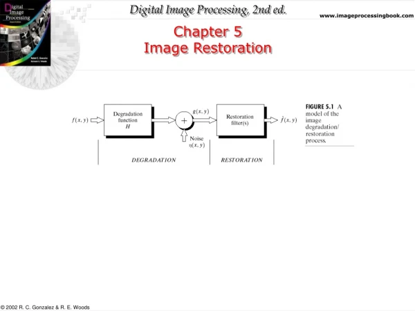
2. Model of Image Degradation / Restoration Process • In this model, we assume that there is an additive noise term, operating on an input image f(x,y) to produce a degraded image g(x,y). • Given g(x,y) and some information about degradation function H, and knowledge about noise term η(x,y). • The aim of restoration is to get an estimate f(x,y) of original image. • The more we know about H and term η, we get better results.

3. Model of Image Degradation / Restoration Process • Here H is a linear, position-invariant process. The degraded image is given as: • g(x,y) = h(x,y)*f(x,y) + η(x,y) • Here h(x,y) is the spatial representation of the degradation function. • The symbol * indicates convolution. • The convolution in spatial domain is equal to multiplication in frequency domain. • In Frequency domain we have: • G(u,v) = H(u,v)F(u,v) + N(u,v) • Here capital letters are the Fourier transforms of the corresponding terms. • For simplicity, we consider the case of H being the identity operator.

5. Origin of Noise • Noise in a digital image arises mainly due to acquisition (digitization) and / or transmission. • Environmental conditions, quality of sensing elements, interference in the transmission channel, lightning and atmospheric disturbance are some examples.

6. Properties of Noise • When the Fourier spectrum of noise is constant, the noise is called a white noise. • This is similar to white light, which contains nearly all frequencies in the visible spectrum in equal quantities. • Fourier spectrum of a function containing all frequencies in equal proportions is a constant. • We assume that noise is independent of coordinates, and it is uncorrelated with respect to the pixel values.

7. Noise Probability Density Functions • The noise component is considered to be a random variable and characterized by a probability density function (PDF). • Some common PDFs used in image processing are: • Gaussian noise • Gaussian (or normal) noise wide spread in usage. The PDF of a Gaussian random variable, z is given by • p(z) = (1/sqrt(2*Л*σ)).exp (-(z-μ)2/2* σ2) • Here z represents gray level, μ is the mean of z, and σ is the standard deviation. • The square of standard deviation is called the variance of z. • Nearly 70% of the value of this function lies in the range [(μ – σ), (μ + σ)] and about 95% of its value lies in the range [(μ –2 σ), (μ + 2σ)].

9. % Gaussian noise % Read a gray scale image (having few regulat patterns) and add gaussian % noise of certain mean value,standard deviation and certain percentage. % plot the histogram of noise, noisy image. ensure that the profile of the % noise is visible in the profile of the noisy image. clear all; close all; clc; a = imread('pattern.png'); a = im2double(a); sizeA = size(a); p3 = 0; % Gaussian noise mean value p4 = 1; % Gaussian noise variance value R = p3+p4*randn([256,256]); R1 = a+R; figure,imshow(R1),title('Noisy Image'); figure,hist(R,50),title('Probability density function');

10. Rayleigh noise • The PDF of Rayleigh noise is given by • p(z) = (2/b)*(z-a)*exp(-(z-a)2/b for z ≥ a • = 0 for z < a • The mean and variance of this PDF are: • μ = a + sqrt(Πb/4) and σ2 = b(r – Π)/4. • One has to note the displacement of PDF from the origin and skewed to the right. • Thus this is useful for skewed histograms.

12. % Rayleigh noise % Read a gray scale image (having few regulat patterns) and add rayleigh % noise of certain mean value,standard deviation and certain percentage. % plot the histogram of noise, noisy image. ensure that the profile of the % noise is visible in the profile of the noisy image. clear all; close all; clc; a = imread('pattern.png'); a = im2double(a); sizeA = size(a); p3 = 0.95; A = 0; B = 2; R = A + (-B*log(1-rand(sizeA))).^0.5; x = rand(sizeA); b=a; for i=1:sizeA(1) for j=1:sizeA(2) if (x(i,j)< p3) b(i,j)=a(i,j)+R(i,j); end end end figure,imshow(a); figure,imshow(b),title('Noisy Image'); figure,hist(R,50),title('Probability density function'); figure,hist(b);

13. Erlang (Gamma) noise • The PDF of Erlang noise is given by • abzb-1 • p(z) = -------- e-az for z ≥ 0 • (b -1) ! • = 0 for z < 0 • Here a > 0, b is a positive integer. The mean and variance of this density are: • μ = (b/a) and σ2 = (b/a2).

15. % erlang noise % Read a gray scale image (having few regulat patterns) and add erlang % noise of certain mean value,standard deviation and certain percentage. % plot the histogram of noise, noisy image. ensure that the profile of the % noise is visible in the profile of the noisy image. clear all; close all; clc; a = imread('pattern.png'); a = im2double(a); sizeA = size(a); p3 = 0.9; A = 2; B = 5; k = -1/A; R = zeros(sizeA); for i=1:B R = R+k*log(1-rand(sizeA)); end x = rand(sizeA); b=a; for i=1:sizeA(1) for j=1:sizeA(2) if (x(i,j)< p3) b(i,j)=a(i,j)+R(i,j); end end end figure,imshow(a); figure,imshow(b),title('Noisy Image'); figure,hist(R,50),title('Probability density function'); figure,hist(b);

16. Exponential noise • The PDF of exponential noise is given as: • p(z) = ae-az for z ≥ 0 • = 0 for z < 0 • Here a > 0. The mean and variance of this density function are • μ = (1/a) and σ2 = (1/a2). • This PDF is the special case of the Erlang PDF, with b =1.

18. % Exponential noise % Read a gray scale image (having few regulat patterns) and add exponential % noise of certain mean value,standard deviation and certain percentage. % plot the histogram of noise, noisy image. ensure that the profile of the % noise is visible in the profile of the noisy image. clear all; close all; clc; a = imread('pattern.png'); a = im2double(a); sizeA = size(a); p3 = 0.9; A = 1; k = -1/A; R = k*log(1-rand(sizeA)); x = rand(sizeA); b=a; for i=1:sizeA(1) for j=1:sizeA(2) if (x(i,j)< p3) b(i,j)=a(i,j)+R(i,j); end end end figure,imshow(a); figure,imshow(b),title('Noisy Image'); figure,hist(R,50),title('Probability density function'); figure,hist(b);

19. Uniform noise • The PDF of uniform noise is given by: • p(z) = (1/(b-a)) if a ≤ z ≤ b • = 0 otherwise • The mean and variance are given as: • μ = (a+b)/2 and σ2 = ((b-a)2)/12.

21. % Uniform noise % Read a gray scale image (having few regulat patterns) and add uniform % noise of certain mean value,standard deviation and certain percentage. % plot the histogram of noise, noisy image. ensure that the profile of the % noise is visible in the profile of the noisy image. clear all; close all; clc; a = imread('pattern.png'); %a = zeros([256,256]); a = im2double(a); sizeA = size(a); A = 0; % Min noise level B = 1; % Max noise level p3 = 0.95; % Noise percentage R = A + (B - A)*rand(sizeA); x = rand(sizeA); b=a; for i=1:sizeA(1) for j=1:sizeA(2) if x(i,j) < p3 b(i,j)=a(i,j)+R(i,j); end end end figure,imshow(a); figure,imshow(b),title('Noisy Image'); figure,hist(R,50),title('Probability density function'); figure,hist(b);

22. Impulse ( salt and pepper) noise • The PDF of (bipolar) impulse noise is given by: • p(z) = Pa for z = a • = Pb for z = b • = 0 otherwise • If b > a, gray-level b will appear as a light dot in the image. Level a will appear like a dark dot. • If either Pa or Pb is zero, the impulse noise is called unipolar. • If both the probabilities are equal, impulse noise will resemble salt and pepper noise. • Hence bipolar noise is also called as salt-and-pepper noise or Shot and spike noise.

23. Impulse Noise • Noise impulses can be positive or negative. • Generally impulse corruption is large compared to the strength of image signal and hence are treated as extreme (black or white) values. • Negative impulses appear s black (pepper) points. • Positive impulses appear white (salt) noise. • For an 8 bit image a = 0 (black) and b = 255 (white).

25. % Salt & pepper noise noise % Read a gray scale image (having few regulat patterns) and add salt & % pepper noise of certain mean value,standard deviation and certain percentage. % plot the histogram of noise, noisy image. ensure that the profile of the % noise is visible in the profile of the noisy image. clear all; close all; clc; %a = imread('pattern.png'); a = zeros([256,256]); a = im2double(a); sizeA = size(a); p3 = 0.3; b = a; x = rand(sizeA); b(x < p3/2) = 0; % Minimum value b(x >= p3/2 & x < p3) = 1; % Maximum (saturated) value figure,imshow(a); figure,imshow(b),title('Noisy Image'); figure,hist(b,50),title('Probability density function');

26. Origin of Noises • Gaussian noise arises in an image such as electronic circuit noise and sensor noise due to poor illumination and/or high temperature. • The Rayleigh noise arises in range imaging. • The exponential and gamma noises appear in laser imaging. • Impulse noise is found in places where quick transients, such as faulty switching take place during imaging.

27. Restoring Noisy images in spatial domain • Spatial filtering is good when only additive noise is present. • Arithmetic mean filter • Let Sxy represent the set of coordinates in a rectangular subimage window of size m X n, centered at (x,y). • The arithmetic mean filter computes the average value of the corrupted image g(x,y) in the area of Sxy. • The restored image f’ at any point (x,y) is the arithmetic mean calculated using the region of Sxy. Thus, • f’(x,y) = (1/mn) * Σ g(s,t) • This operation is carried on a convolution mask in which all coefficients have the value (1/mn). • This filter simply smoothes local variations in an image. • Noise is reduce as a result of blurring.

28. Geometric mean filter • This filter can be implemented using the expression: • f’(x,y) = [ Π g(s,t) ]1/mn • Here each restored pixel is given by the product of the pixels in the subimage window, raised to the power of 1/mn. • It gives smoothing comparable to that of arithmetic mean filter, but tends to lose less image detail during the process.

30. Harmonic mean filter • This filter can be given by: • f’(x,y) = (mn) / Σ (1/g(s,t)). • This filter is good for removing salt noise. • But fails to remove pepper noise. • It works well with other noises such as Gaussian noise.

32. % Harmonic mean filter % Read a gray scale image and add a noise to it and filter it using % Harmonic mean filter. clear all; close all; clc; f = imread('Saltcman.tif'); %f = imnoise(f,'gaussian',0,0.02); f = im2double(f); %subplot(1,2,1),imshow(f),title('Original Image'); figure,imshow(f),title('Salt Noise'); [m n]=size(f); for i = 2:m-1 for j = 2:n-1 con=0; s1=0; for k1 = i-1:i+1 for p1 = j-1:j+1 con = con+1; if f(k1,p1)==0 s1 = s1+0; else s1=s1+(1/f(k1,p1)); end end end b1(i,j)=con/s1; end end %subplot(1,2,2),imshow(b1),title('Harmonic mean filtered'); figure,imshow(b1),title('Harmonic mean filtered');

33. Contra harmonic mean filter • This filer can be implemented using the expression: • f’(x,y) = Σ g(s,t)Q+1/Σ g(s,t)Q • Here Q is the order of the filter. • It is good for reducing the effect of salt and pepper noise. • For positive values of Q, it eliminates pepper noise and for negative values of Q it eliminates salt noise. • It reduces to arithmetic mean filter for Q = 0 and harmonic mean filter for Q = -1. • Generally, the positive order filter cleans the background, by blurring dark areas.

34. Contra harmonic mean filter • Arithmetic and geometric mean filters are good for removing random noise like Gaussian or uniform noise. • Contraharmonic filer is good for impulse noise. • But it must be known before hand that whether the noise is dark or light to fix the Q value.

36. % Contraharmonic mean filter % Read a gray scale image and applay contraharmonic filter for verious Q % values. prove that for negative values of Q salt noise is removed, for % positive values of Q pepper noise is removed. check that % for Q=0 it becomes mean filter and for Q=-1 it becomes harmonic filter. clear all; close all; clc; f = imread('Peppercman.tif'); %f = imnoise(f,'salt & pepper',0.1); f = im2double(f); %subplot(1,2,1),imshow(f),title('Original Image'); figure,imshow(f),title('Pepper Noise'); [m n]=size(f); Q=1; for i = 2:m-1 for j = 2:n-1 con=0; s1=0; s2=0; for k1 = i-1:i+1 for p1 = j-1:j+1 con = con+1; s1=s1+(f(k1,p1)^Q); s2=s2+(f(k1,p1)^(Q+1)); end end b1(i,j)=s2/s1; end end %subplot(1,2,2),imshow(b1),title('Cantraharmonic mean filtered'); figure,imshow(b1),title('Contraharmonic mean filtered');

37. Order Statistics Filter • These are spatial filters whose response is based on ordering (ranking) the pixels in the image area encompassed by the filter. • Median filter • Here we replace the value of a pixel by the median of the gray values in the neighborhood of that pixel: • f’(x,y) = median {g(s,t)} • The original value of the pixel is included in the calculation of the median. • For some types of random noise, they give excellent noise-reduction with less blurring than linear smoothing filters of same size. • They work well with unipolar and bipolar impulse noises.

39. Max and min filters • Median is the 50th percentile of a ranked set of numbers. The 100th percentile results in max filter given as: • f’(x,y) = max {g(s,t)} • This filter is useful in finding the brightest spots in an image. • As pepper noise has very low intensity values, they are reduced by this filter. • The 0th percentile filter is the min filter: • f’(x,y) = min {g(s,t)} • this filter is capable of identifying the darkest points in an image. • It reducecs salt noise as a result of min operation.

42. % Max and Min filters % Read a gray scale image and add salt & pepper noise and remove the same % with min filter and max filter. clear all; close all; clc; f = imread('cameraman.tif'); f = imnoise(f,'salt & pepper',0.01); f = im2double(f); %subplot(2,2,1),imshow(f),title('Original Image'); figure,imshow(f),title('Noisy Image'); [m n]=size(f); Q=0; for i = 2:m-1 for j = 1:n-1 con=0; for k1 = i-1:i+1 for p1 = j-1:j+1 con = con+1; s1(con)=(f(k1,p1)); end end b1(i,j)=min(s1); b2(i,j)=max(s1); end end %subplot(2,2,2),imshow(b1),title('Min filter'); %subplot(2,2,3),imshow(b2),title('Max filter'); figure,imshow(b1),title('Min filter'); figure,imshow(b2),title('Max filter');

43. Midpoint filter • This filter is simply the midpoint between the maximum and minimum values in the area enclosed by the filter: • f’(x,y) = (1/2) * [ max {g(s,t)} + min {g(s,t)}] • This filter combines order statistic and averaging. • It is good for randomly distributed noise, like Gaussian or uniform noise.

45. % Midpoint filter % Read a gray scale image and add gaussian noise and remove the noise using % midpoint filter clear all; close all; clc; f = imread('cameraman.tif'); f = imnoise(f,'gaussian',0,0.01); f = im2double(f); %subplot(1,2,1),imshow(f),title('Noisy Image'); figure,imshow(f),title('Noisy Image'); [m n]=size(f); Q=0; for i = 2:m-1 for j = 2:n-1 con=0; for k1 = i-1:i+1 for p1 = j-1:j+1 con = con+1; s1(con)=(f(k1,p1)); end end b1=min(s1); b2=max(s1); R_img(i,j)=(b1+b2)/2; end end %subplot(1,2,2),imshow(R_img),title('Midpoint filtered'); figure,imshow(R_img),title('Midpoint filtered');

46. Alpha trimmed mean filter • Let us delete the d/2 lowest and the d/2 highest gray-level values of g(s,t) in the neighborhood of Sxy. • Let gr(s,t) represent the remaining (mn – d ) pixels. • A filter formed by averaging these remaining pixels is called an alpha-trimmed mean filter: • f’(x,y) = (1/(mn-d))* Σ gr(s,t) • Here the value of d can vary from 0 to (mn – 1). • When d = 0, it reduces to arithmetic mean filter. • For d = (mn-1)/2, it becomes a median filter. • For other values of d, it is useful in situations involving multiple types of noise, such as combination of salt and pepper and Gaussian noise.

48. % read a gray scale image and remove the salt & pepper noise using alpha % trimed mean filter. prove that for D=0 it becomes arithmetic mean filter % and for d=(mn-1)/2 it becomes median filter. show that this filter % removes combination of gaussian and salt & pepper noise. clear all; close all; clc; f = imread('cameraman.tif'); f = im2double(f); f = imnoise(f,'salt & pepper',0.1); f = imnoise(f,'gaussian',0,0.01); [m n]=size(f); f1=zeros(m,n); D = 4; d = D/2; for i=3:m-2 for j=3:n-2 con=0; for k=i-2:i+2 for p=j-2:j+2 con=con+1; s(con)=f(k,p); end end s = sort(s); r = (size(s,2)-d); s1= s(d+1:r); f1(i,j)= sum(s1)/(con-D); end end figure,imshow(f),title('Noisy Image'); figure,imshow(f1),title('Alpha-trimmed mean filter');

49. Adaptive filters • The filters discussed above, do not worry about the image characteristics. • Adaptive filters are one whose behavior changes based on statistical characteristics of the image inside the filter region defined by the m X n subimage. • Adaptive, local noise reduction filter • Mean and variance are the simple statistical feature of a random variable. • They are related to the appearance of an image. • Mean gives a measure of average gray level in the region over which the mean is computed and variance gives a measure of average contrast in that region.

50. Response of a filter • The response of a filter at (x,y) depends on: • g(x,y), the value of the noisy image at (x,y). • ση2, the variance of the noise corrupting the image f(x,y) • mL, the local mean of the pixels in Sxy. • σL2, the local variance of the pixels in Sxy.