Image Restoration

1. Image Restoration

2. Image Restoration • Image restoration vs. image enhancement • Enhancement: • largely a subjective process • Priori knowledge about the degradation is not a must (sometimes no degradation is involved) • Procedures are heuristic and take advantage of the psychophysical aspects of human visual system • Restoration: • more an objective process • Images are degraded • Tries to recover the images by using the knowledge about the degradation

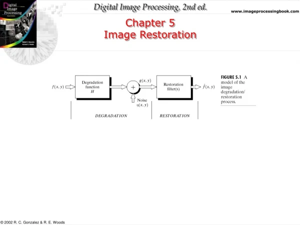
3. An Image Degradation Model • Two types of degradation • Additive noise • Spatial domain restoration (denoising) techniques are preferred • Image blur • Frequency domain methods are preferred • We model the degradation process by a degradation function h(x,y), an additive noise term, (x,y), as g(x,y)=h(x,y)*f(x,y)+ (x,y) • f(x,y) is the (input) image free from any degradation • g(x,y) is the degraded image • * is the convolution operator • The goal is to obtain an estimate of f(x,y) according to the knowledge about the degradation function h and the additive noise  • In frequency domain: G(u,v)=H(u,v)F(u,v)+N(u,v) • Three cases are considered • g(x,y)=f(x,y)+ (x,y) • g(x,y)=h(x,y)*f(x,y) • g(x,y)=h(x,y)*f(x,y)+ (x,y)

4. A Model of the Image Degradation/Restoration Process

5. Noise Model • We first consider the degradation due to noise only • h is an impulse for now ( H is a constant) • White noise • Autocorrelation function is an impulse function multiplied by a constant • It means there is no correlation between any two pixels in the noise image • There is no way to predict the next noise value • The spectrum of the autocorrelation function is a constant (white)

6. Gaussian Noise • Noise (image) can be classified according the distribution of the values of pixels (of the noise image) or its (normalized) histogram • Gaussian noise is characterized by two parameters,  (mean) and σ2 (variance), by • 70% values of z fall in the range [(-σ),(+σ)] • 95% values of z fall in the range [(-2σ),(+2σ)]

7. Gaussian Noise H.R. Pourreza

8. Other Noise Models • Rayleigh noise • The mean and variance of this density are given by • a and b can be obtained through mean and variance

9. Other Noise Models • Erlang (Gamma) noise • The mean and variance of this density are given by • a and b can be obtained through mean and variance

10. Other Noise Models • Exponential noise • The mean and variance of this density are given by • Special case pf Erlang PDF with b=1

11. Other Noise Models • Uniform noise • The mean and variance of this density are given by

12. Other Noise Models • Impulse (salt-and-pepper) noise • If either Pa or Pb is zero, the impulse noise is called unipolar • a and b usually are extreme values because impulse corruption is usually large compared with the strength of the image signal • It is the only type of noise that can be distinguished from others visually

13. A Sample Image

14. Effect of Adding Noise to Sample Image

15. Effect of Adding Noise to Sample Image

16. Periodic Noise • Arises typically from electrical or electromechanical interference during image acquisition • It can be observed by visual inspection both in the spatial domain and frequency domain • The only spatially dependent noise will be considered

17. Estimation of Noise Parameters • Periodic noise • Parameters can be estimated by inspection of the spectrum • Noise PDFs • From sensor specifications • If imaging sensors are available, capture a set of images of plain environments • If only noisy images are available, parameters of the PDF involved can be estimated from small patches of constant regions of the noisy images

19. Estimation of Noise Parameters • In most cases, only mean and variance are to be estimated • Others can be obtained from the estimated mean and variance • Assume a sub-image with plain scene is available and is denoted by S

20. Restoration in the Presence of Noise Only (De-Noising) • Mean filters • Arithmetic mean filter • g(x,y) is the corrupted image • Sx,y is the mask • Geometric mean filters • Tends to preserve more details • Harmonic mean filter • Works well for salt noise but fails for pepper noise • Contraharmonic mean filter • Q: order of the filter • Positive Q works for pepper noise • Negative Q works for salt noise • Q=0arithmetic mean filter • Q=-1harmonic mean filter

21. De-Noising Corrupted by Gaussian Noise Mean Filtering Geometric Mean Filtering

22. De-Noising Corrupted by pepper noise Corrupted by salt noise 3x3 Contraharmonic Q=1.5 3x3 Contraharmonic Q=-1.5

23. De-Noising

24. Filters Based on Order Statistics(De-Noising) • Median filter • Median represents the 50th percentile of a ranked set of numbers • Max and min filter • Max filter uses the 100th percentile of a ranked set of numbers • Good for removing pepper noise • Min filter uses the 1 percentile of a ranked set of numbers • Good for removing salt noise • Midpoint filter • Works best for noise with symmetric PDF like Gaussian or uniform noise

25. De-Noising One pass median filtering Corrupted by salt & pepper noise Three pass median filtering Two pass median filtering

26. Corrupted by pepper noise Corrupted by salt noise De-Noising Max Filtering Min Filtering

27. Alpha-Trimmed Mean Filter(De-Noising) • Alpha-trimmed mean filter takes the mean value of the pixels enclosed by an m×n mask after deleting the pixels with the d/2 lowest and the d/2 highest gray-level values • gr(s,t) represent the remaining mn-d pixels • It is useful in situations involving multiple types of noise like a combination of salt-and-pepper and Gaussian

28. De-Noising Added salt & pepper noise Corrupted by additive Uniform noise 5x5 Mean Filtering 5x5 Geo-Mean Filtering 5x5 Median Filtering 5x5 Alpha-trimmed Mean Filtering H.R. Pourreza

29. Adaptive Filters(De-Noising) • Adaptive Local Noise Reduction Filter • Assume the variance of the noise is either known or can be estimated satisfactorily • Filtering operation changes at different regions of an image according to local variance calculated within an M×N region • If , the filtering operation is defined as • If , the output takes the mean value • That is: • At edges, it is assumes that

30. De-Noising Corrupted by Gaussian noise Mean Filtering Adaptive Filtering Geo-Mean Filtering

31. Adaptive Median Filter(De-Noising) • Median filter is effective for removing salt-and-pepper noise • The density of the impulse noise can not be too large • Adaptive median filter • Notation • Zmin: minimum gray value in Sxy • Zmax: maximum gray value in Sxy • Zmed: median of gray levels in Sxy • Zxy: gray value of the image at (x,y) • Smax: maximum allowed size of Sxy

32. Adaptive Median Filter(De-Noising) • Two levels of operations • Level A: • A1= Zmed –Zmin • A2= Zmed –Zmax • If A1 > 0 AND A2 < 0, Go to level B else increase the window size by 2 • If window size <= Smax repeat level A else output Zxy • Level B: • B1= Zxy –Zmin • B2= Zxy –Zmax • If B1 > 0 AND B2 < 0, output Zxy else output Zmed Used to test whether Zmed is part of s-and-p noise. If yes, window size is increased Used to test whether Zxy is part of s-and-p noise. If yes, apply regular median filtering

33. De-Noising Median Filtering Adaptive Median Filtering

34. Linear, Position-Invariant Degradation • Degradation Model In the absence of additive noise: For scalar values of a and b, H is linear if: H is Position-Invariant if:

35. Linear, Position-Invariant Degradation In the presence of additive noise: • Many types of degradation can be approximated by linear, position-invariant processes • Extensive tools of linear system theory are available • In this situation, restoration is image deconvolution

36. Estimating the Degradation Function • Principal way to estimate the degradation function for use in image restoration: • Observation • Experimentation • Mathematical modeling

37. Estimating by Image Observation • We look for a small section of the image that has strong signal content ( ) and then construct an un-degradation of this section by using sample gray levels ( ). Now, we construct a function on a large scale, but having the same shape.

38. Estimating by Experimentation • We try to obtain impulse response of the degradation by imaging an impulse (small dot of light) using the system. Therefore

39. Estimating by Modeling Atmospheric turbulence model: High turbulence k=0.0025 Negligible turbulence Low turbulence k=0.00025 Mid turbulence k=0.001 H.R. Pourreza

40. Estimating by Modeling Blurring by linear motion:

41. Estimating by Modeling H.R. Pourreza

42. Inverse Filtering The simplest approach to restoration is direct inverse filtering: Even if we know the degradation function, we cannot recover the un-degraded image If the degradation has zero or very small values, then the ratio N/H could easily dominate our estimation of F . One approach to get around the zero or small-value problem is to limit the filter frequencies to value near the origin.

43. Inverse Filtering Degraded Image Filtering with H cut off outside a radius of 40 Full inverse Filtering Filtering with H cut off outside a radius of 70 Filtering with H cut off outside a radius of 85 H.R. Pourreza

44. Minimum Mean Square Error Filtering(Wiener Filtering) This approach incorporate both the degradation function and statistical characteristic of noise into the restoration process. Image and noise are random process The objective is to find an estimation for f such that minimized e2

45. Minimum Mean Square Error Filtering(Wiener Filtering) If the noise is zero, then the Wiener Filter reduces to the inverse filter.

46. Minimum Mean Square Error Filtering(Wiener Filtering) Unknown Constant

47. Wiener Filtering Wiener filtering (K was chosen interactively) Radially limited inverse filtering Full inverse filtering

48. Wiener Filtering Inverse filtering Wiener filtering Reduced noise variance H.R. Pourreza