Ch5 Image Restoration

1. Ch5 Image Restoration CS446 Instructor: Nada ALZaben

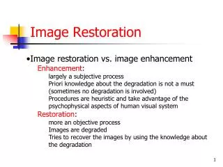
2. Image restoration • Restoration attempts to reconstruct or recover an image that has been degraded by using a prior knowledge of the degradation phenomenon • Restoration techniques are oriented toward modeling the degradation and applying the inverse process in order to recover the original image • Some restoration techniques are best formulated in the spatial domain, while others are better suited for the frequency domain

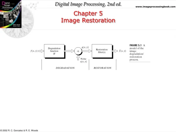
3. A model of the Image Degradation/Restoration Process [1] • The degradation process: modeled as a degradation function H together with an additive noise term operates on an input image f(x,y) to produce a degraded image g(x,y) • Given knowledge about the additive noise term n(x,y), the objective of restoration is to obtain an estimate f’(x,y) of the original input image

4. A model of the Image Degradation/Restoration Process [2] • If H is a linear position-invariant process then the degraded image is given in the spatial domain by: g(x,y) = h(x,y) * f(x,y) + n(x,y) • Where: h(x,y) is the spatial representation of the degradation function and * indicates convolution • We may also write the model in the frequency domain representation: G(u,v) = H(u,v) F(u,v) + N(u,v) • Where the terms in capital letters are the Fourier transform of the corresponding terms in the previous equation • We will assume that H is the identity operator and we deal only with degradation due to noise

5. Noise Model • The principle sources of noise in digital images arise during image acquisition (digitization) and/or transmission • Frequency properties refer to the frequency content of noise in the Fourier sense • when the Fourier spectrum of noise is constant the noise usually is called white noise • We will assume that noise is independent of spatial coordinates and that it is uncorrelated with respect to the image itself (i.e. no correlation between pixel values and the values of noise components)

6. Some Important Noise Probability Density Functions (PDF) • The spatial noise descriptor is the statistical behavior of the gray-level values in the noise component of the model • These may be characterized by a probability density function PDF • The most common PDFs in image processing: • Gaussian noise • Impulse noise (salt and pepper) • Gamma noise … etc

7. Gaussian Noise • Gaussian (also called normal) noise models are frequently used in practice • The PDF of a Gaussian random variable z is given by: • Where: z represent gray level, µ is the mean of average value of z and σ is its standard deviation

8. Impulse (Salt and Pepper) Noise • The PDF of impulse (bipolar) noise given by: • If b > a: • Gray level b will appear as a light dot in the image • Level a will appear like a dark dot • If either Pa or Pb is zero, the impulse noise is called unipolar noise • If neither Pa or Pb is zero, and if they are approximately equal the impulse noise is called salt and pepper. • For an 8-bit image a = 0 (black) and b = 255 (white)

10. Mean Filters • Arithmetic mean filter: • let Sxy be the set of coordinates in a rectangualrsubimage window of size mxn centered at point (x,y), • The arithmetic mean filtering process computes the average of the corrupted image g(x,y) in the area defined by Sxy: • The operation can be implemented using a convolution mask in which all coefficients = 1/mn

11. Mean Filters • Geometric mean filter: • is given by the expression: • Achieves smoothing comparable to the arithmetic mean filter but it tends to lose less image detail in the process

12. Mean Filters • Harmonic mean filter: • Works well for salt noise but fails for pepper noise • It does well also with other types of noise. • Contraharmonic mean filter: • Well suited for reducing the effect of salt-and-pepper noise

15. Order-Statistic Filters • Median filter: • Practically effective in the presence of both bipolar and unipolar impulse noise • Max and min filters: • Max: useful for finding the brightest points in an image (pepper noise reduced) • Min: useful for finding the darkest points (reduces salt) • Midpoint filter: • Computes the midpoint between the maximum and minimum values in the area encompassed by the filter • Works best for randomly distributed noise

17. Adaptive Filters • Adaptive filters are filters whose behavior changes based on statistical characteristics of the image inside the filter region defined by the m × n rectangular window Sxy • They are capable of performance superior to that of the filters discussed thus far

18. Adaptive Median Filter • The median filter performs well as long as the spatial density of the impulse noise is not large (as a rule of thump, Pa and Pb less than 0.2) • Adaptive median filter • can handle impulse noise with larger probabilities • And it seeks to preserve detail while smoothing nonimpulse noise • The adaptive median filter works in a rectangular window area Sxy, but it changes the size of Sxy during filter operation • Keep in mind: The output of the filter is a single value used to replace the value of the pixel at (x,y)

19. Adaptive Median Filter • It have three main purposes: • To remove salt and-pepper (impulse) noise • Provide smoothing of other noise (may not be impulsive) • Reduce distortion such as excessive thinning or thickening of object boundaries • Consider the following notation: • zmin = minimum gray level value in Sxy • zmax = maximum gray level value in Sxy • zmed = median of gray levels in Sxy • zxy = gray level at coordinates (x,y) • Smax = maximum allowed size of Sxy

20. Adaptive Median Filter • The adaptive median filtering algorithm works in two levels, denoted as level A and level B, as follows: • Level A: • A1 = zmed – zmin • A2 = zmed – zmax • If A1 > 0 AND A2 < 0 • Go to level B • Else increase the window size • If window size ≤ Sxy • repeat level A • Else output zxy • Level B: • B1 = zxy – zmin • B2 = zxy – zmax • If B1 > 0 AND B2 < 0 • Output zxy • Else output zmed

22. Resource • R.C. Gonzalez and R.E. Woods, Digital Image Processing, 2rd Edition, Prentice Hall