Download
1 / 44
440 likes | 628 Vues
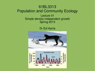
Lecture 03 Density dependent population growth and intra-specific competition Spring 2013 Dr Ed Harris. 61BL3313 Population and Community Ecology. Announcements -lecture + tutorial -issues, comments?. Today carry on with K! -density dependence with discrete generations

E N D
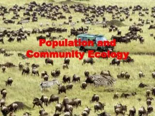
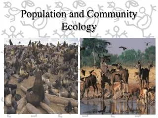
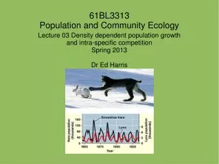
Lecture 03 Density dependent population growth and intra-specific competition Spring 2013 Dr Ed Harris 61BL3313Population and Community Ecology
Announcements -lecture + tutorial -issues, comments?
Today carry on with K! -density dependence with discrete generations -density dependence with overlapping generations -non-linear dd and the Allee effect -time lags and limit cycles -chaos and stochasticity -field data -behaviour and intraspecific competition
review intro logistic population growth with density dependence
review intro logistic population growth with density dependence -more realistic than DI growth -lots of evideince in lab and field to support this idea -ignores competing different species, predators, etc.
density dependence with discrete generations -remember the discrete generation equation without DD -with density dependence, we expect R to decrease as the population approaches the carrying capacity, K -how to incorporate?
density dependence with discrete generations -the basic approach is to divide the regular equation above by the potential population increase relative to the carrying capacity -the population should grow at the rate of R when it is very small -the population should grow more slowly as N approaches the carrying capacity K
density dependence with discrete generations (Nt)(R-1) is the potential increase K is the carrying capacity
density dependence with discrete generations if we do this: we can rearrange the equation...
density dependence with discrete generations to this: You can see "a prime" stays constant and small pop growth slows as Nt grows
density dependence with discrete generations can also think of it as:
density dependence with discrete generations R code: Na <- c(100,120,144,173,207,249,299,358,430,516,619,743,892,1070,1284) Nb <- c(100,118,138,161,187,217,249,285,323,364,408,452,498,543,588) time <- c(0:14) plot(time, Na, ylim=c(0,1300), main="Density-independent") plot(time, Nb, ylim=c(0,1300), main="Density-dependent")
density dependence with overlapping generations start with our recent friend:
density dependence with overlapping generations and as we discussed earlier:
density dependence with overlapping generations DD population growth based on the logistic equation
density dependence with overlapping generations lots of animals show this kind of growth both in the lab (e.g., the Paramecium) and in the field:
density dependence with overlapping generations assumptions for this model: 1 The carrying capacity is a constant; 2 population growth is not affected by the age distribution; 3 birth and death rates change linearly with population size (it is assumed that birth rates and survivorship rates both decrease with density, and that these changes follow a linear trajectory);
density dependence with overlapping generations assumptions for this model: 4 the interaction between the population and the carrying capacity of the environment is instantaneous: that is, the population is “sensitive” to the carrying capacity with no time lags; 5 abiotic, density-independent factors do not affect birth and death rates (no environmental stochasticity); 6 crowding affects all members of the population equally.
non-linear dd and the Allee effect -until now we've assumed that birth and death rates vary linearly with population density -there is pretty good lab and field evidence that this is often not true -however this seems to rarely have a strong effect on actual observed population growth -a major exception is the "Allee effect"
non-linear dd and the Allee effect -the idea here is that there is some minimum viable population (MVP) size for a given population -below this size, birth/death rates decrease/increase making extinction very likely
Allee effect What causes this effect?
non-linear dd and the Allee effect (i) group cooperation reduces losses from predators; (ii) group foraging for food is more efficient (foraging facilitation); (iii) small populations are more subject to density-independent or stochastic extinctions as well as genetic effects such as inbreeding depression; (iv) Low birth rates in small populations could result from pollination failure in plants; (v)male and female animals unable to locate each other, or the chance of a very unequal sex ratio (large number of males, few females).
time lags and limit cycles -one of the assumtions of the logistic DD growth model above is that populations respond immediately to the carrying capacity -this probably is not true, especially for populations that have high potential for fast reproduction -what is predicted therefore is that population size will "overshoot" K, then compensate below K -an ocillation of population size around K should be observed
time lags and limit cycles -we can easily modify the discrete logistic growth equation to look at this -the Tau (T) in the exponent is the magnitude of time that the population lags in responding to K
time lags and limit cycles -the product of r and T determines the behaviour of the population over time
chaos and stochasticity -if growth rate in a population is very large (e.g. r > 2), population growth has been shown to behave chaotically -here are a few examples to illustrate
chaos and stochasticity (discrete logistic growth model) r < 2.0
chaos and stochasticity (discrete logistic growth model) r =2.2, 2-point cycle
chaos and stochasticity (discrete logistic growth model) r =2.6, 4-point cycle
chaos and stochasticity (discrete logistic growth model) r =2.75, chaos
field data -according to discussion above, an increase in population density might be predicted to:
field data American bison typical grazer huge pop'n density
field data I digress: ~60,000,000 in 1800 ~750 in 1890
field data Birth rate of the American bison (Bison bison) as a function of population size. After Fowler (1981)
field data American "elk" 2nd biggest deer
field data Recruitment of elk (Cervus elaphus) calves in Yellowstone National Park as a function of adult population size in the previous year. Based on Houston (1982)