Introduction to Robotics
340 likes | 597 Vues
Introduction to Robotics. Alfred Bruckstein Yaniv Altshuler. Course. 4 Home assignments (10% each) Final exam (60%). Plan. Introduction and mathematical tools Forward kinematics Inverse kinematics Navigation Multi robotics. Bibliography.

Introduction to Robotics
E N D
Presentation Transcript
Introduction to Robotics Alfred Bruckstein Yaniv Altshuler
Course • 4 Home assignments (10% each) • Final exam (60%)
Plan • Introduction and mathematical tools • Forward kinematics • Inverse kinematics • Navigation • Multi robotics
Bibliography • Physics-Based Animation, Kenny Erleben , Jon Sporring , Knud Henriksen , Henrik Dohlmann, Charles River Media 2005
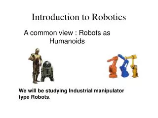
Robots are artificial physical or virtual/software agents that can sense and interact with environment using theirsensors and effectors. Introduction Czech playwright Karel Capek in 1921 described a robot (from robota = work, labour) - a machine resembling humans and which can work without effort.
Introduction:type of robots Most of physical robots fall into one of the three categories: • Manipulators/robotic arms which are anchored to their workplace and built usually from sets of rigid links connected by joints. • Mobile robots which can move in their environment using wheels, legs, etc. • Hybrid robots which include humanoid robots are mobile robots equipped with manipulators.
Introduction:types of sensors Traditionally robot sensors can be split into two categories: • Proprioceptive sensors which provide information about robot internal state: configuration of joints (shaft encoders), force and torque measured at robots wrist, battery charge, etc. • Exteroceptive sensors which enables a robot to sense its environment. The group involves imaging sensors (cameras), tactile sensors, range finders, GPS, and many others. Alternatively, sensors can be: • Active – if they involve direct „interaction” with environment to be able to sense it (sonars, range finders). • Passive – if they do not require such interaction (cameras).
Introduction:Articulated figures • Link : a solid rod, cannot change shape nor lenght • Joint : connection between two links (can rotate/translate with several degrees of freedom)
Introduction:effectors part 1 Effectors enabe robots to interact with the environment – i.e. to change their physical configuration. The kinematic state of a robot effector (constructed of rigid bodies) can be uniquely specified by a constant number of parameters called number of degrees of freedom (DOF). The dynamic state involves additionally the rate of change of each parameters. Rigid bodies can have up to 6 DOF which define pose of the body, specified by e.g. Cartesian position (3 DOF) and angular orientation (3 DOF).
Katana 6M180 has only 5 DOF, therefore in general its end-effector cannot be aligned with arbitrary 6 DOF pose of a manipulated object. Introduction:effectors part 2 Set of all end-effector positions which can be reached for some configuration of joint angles is called the reachable workspace. Set of all positionswhich can be reached by the end-effector with arbitrary orientations is called the dextrous workspace.
r workspace Introduction:effectors part 2 Manipulators , r 1 r 4.5 0 50o x = r cos y = r sin
Introduction:effectors part 3 Mobile robots can have more DOF than the number of actuators. For instance, a car has 3 effective degree of freedom, but only 2 controllable degree of freedom. A robot is nonholonomic when it has more effective DOF than controllable DOF, and holonomic if these numbers are the same.
Revolute joints Prismatic joints Spherical joints 1 controllable DOF 1 controllable DOF 3 controllable DOFs Control of robotic manipulators:joints Joints provide a consistent way of connecting arm links. The configuration of each joint is determined by a specific number of DOF, where each DOF is usually driven by attached motor. The most common types of joints are:
Kinematics • How can a robot move ? • Kinematics : “study of the motion of parts, without considering mass or forces”
Kinematics • Kinematics are subdivided in two groups : • forward kinematics • inverse kinematics
Kinematics • Forward kinematics • Knowing the starting point, what’s the final destination ? • Forward kinematics = computing final destination • Easy, and unique.
Kinematics • Inverse kinematics • I have to get there, how do I do it ? • Inverse kinematics = computing how toarrive to a precise final destination • Not easy, and not always unique ! • Additional constraints may be added : • Smoothness • Dynamic limitations • Obstacles
Mathematical tools • A three dimensional point, in the system {A} :
z y x Mathematical tools • The point P is located along the three axes of the coordinate system
Transformations • A rotation matrix :
Transformations • The product : transformation matrix R by vector point P in the system {B} gives us the vector point P in the system {A}
Transformations • Example
Point P x x Point P+v Translation vector v Transformations • With homogeneouscoordinates • Pure translation matrix, of vector v :
Transformations • Combining rotation and translation
Transformations • Example : rotating a frame B relative to a frame A about Z axis by 30° and moving it 10 units in direction of X and 5 units in the direction of Y. What will be the coordinates of a point in frame A if in frame B the point is : [3, 7, 0]T?
Paired Joint Coordinates • Articulated figure = many links and joints • Each joint can move • The motion of linkjand jointj affects the motion of linki and jointi for i > j • Very difficult to describe the motion in a system common to all links and joints ! • Solution : the Paired Joint Coordinates method
Paired Joint Coordinates • Each linki has three predefined orthogonal coordinates systems : • The Body Frame (BFi) • The Inner Frame (IFi) • The Outer Frame (OFi)
Paired Joint Coordinates • The Body Frame (BFi) • Associated with linki • Origin generally at its center of mass
Paired Joint Coordinates • The Inner Frame (IFi) • Associated with linkiand jointi • Origin on the axis of jointi • One axe parallel to the direction of the motion of the joint
Paired Joint Coordinates • The Outer Frame (OFi) • Associated with linkiand jointi+1 • Origin on the axis of jointi+1 • One axe parallel to the direction of the motion of the joint
Paired Joint Coordinates • With this method we can derive transformationsbetween different frames • But it is a general approach, not easy too use