Hidden Markov Model
Understand how Hidden Markov Models can analyze sequential data like speech recognition. Detailed explanations of the problem, analysis methods, and formalization are provided. Explore the Markov assumption and its impact on modeling sequential events effectively.


Hidden Markov Model
E N D
Presentation Transcript
Hidden Markov Model CS570 Lecture Note KAIST This lecture note was made based on the notes of Prof. B.K.Shin(Pukyung Nat’l Univ) and Prof. Wilensky (UCB)
Sequential Data • Often highly variable, but has an embedded structure • Information is contained in the structure
More examples • Text, on-line handwiritng, music notes, DNA sequence, program codes main() { char q=34, n=10, *a=“main() { char q=34, n=10, *a=%c%s%c; printf( a,q,a,q,n);}%c”; printf(a,q,a,n); }
Example: Speech Recognition • Given a sequence of inputs-features of some kind extracted by some hardware, guess the words to which the features correspond. • Hard because features dependent on • Speaker, speed, noise, nearby features(“co-articulation” constraints), word boundaries • “How to wreak a nice beach.” • “How to recognize speech.”
Defining the problem • Find argmax w∈L P(w|y) • y, a string of acoustic features of some form, • w, a string of words, from some fixed vocabulary • L, a language (defined as all possible strings in that language), • Given some features, what is the most probable string the speaker uttered?
Analysis • By Bayes’ rule: P(w|y)= P(w)P(y|w)/P(y) • Since y is the same for different w’s we might choose, the problem reduces to argmaxw∈L P(w)P(y|w) • we need to be able to predict • each possible string in our language • pronunciation, given an utterance.
P(w) where w is an utterance • Problem: There are a very large number of possible utterances! • Indeed, we create new utterances all the time, so we cannot hope to have there probabilities. • So, we will need to make some independence assumptions. • First attempt: Assume that words are uttered independently of one another. • Then P(w) becomes P(w1)… P(wn) , where wi are the individual words in the string. • Easy to estimate these numbers-count the relative frequency words in the language.
Assumptions • However, assumption of independence is pretty bad. • Words don’t just follow each other randomly • Second attempt: Assume each word depends only on the previous word. • E.g., “the” is more likely to be followed by “ball” than by “a”, • despite the fact that “a” would otherwise be a very common, and hence, highly probably word. • Of course, this is still not a great assumption, but it may be a decent approximation
In General • This is typical of lots of problems, in which • we view the probability of some event as dependent on potentially many past events, • of which there too many actual dependencies to deal with. • So we simplify by making assumption that • Each event depends only on previous event, and • it doesn’t make any difference when these events happen • in the sequence.
Speech Example • Representation • X = x1 x2 x3 x4 x5 … xT-1 xT = s p iy iy iy ch ch ch ch
Analysis Methods • Probability-based analysis? • Method I • Observations are independent; no time/order • A poor model for temporal structure • Model size = |V| = N
Analysis methods • Method II • A simple model of ordered sequence • A symbol is dependent only on the immediately preceding: • |V|×|V| matrix model • 50×50 – not very bad … • 105×105 – doubly outrageous!!
Another analysis method • Method III • What you see is a clue to what lies behind and is not known a priori • The source that generated the observation • The source evolves and generates characteristic observation sequences
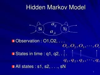
More Formally • We want to know P(w1,….wn-1, wn). • To clarify, let’s write the sequence this way: P(q1=Si, q2=Sj,…, qn-1=Sk, qn=Si) Here the indicate the I-th position of the sequence, and the Si the possible different words from our vocabulary. • E.g., if the string were “The girl saw the boy”, we might have S1= the q1= S1 S2= girl q2= S2 S3= saw q3= S3 S4= boy q4= S1 S1= the q5= S4
Formalization (continue) • We want P(q1=Si, q2=Sj,…, qn-1=Sk, qn=Si) • Let’s break this down as we usually break down a joint : • = P(qn=Si | q1=Sj,…,qn-1=Sk)ⅹP(q1=Sj,…,qn-1=Sk) • … • = P(qn=Si | q1=Sj,…,qn-1=Sk)ⅹP(qn-1=Sk|q1=Sj,…, • qn-1=Sm)ⅹP(q2=Sj|q1=Sj)ⅹP(q1=Si) • Our simplifying assumption is that each event is only • dependent on the previous event, and that we don’t care when • the events happen, I.e., • P(qi=Si | q1=Sj,…,qi-1=Sk)ⅹP(qi=Si | qi-1=Sk)and • P(qi=Si | qi-1=Sk)=P(qj=Si | qj-1=Sk) • This is called the Markov assumption.
Markov Assumption • “The future does not depend on the past, given the present.” • Sometimes this if called the first-order Markov assumption. • second-order assumption would mean that each event depends on the previous two events. • This isn’t really a crucial distinction. • What’s crucial is that there is some limit on how far we are willing to look back.
Morkov Models • The Markov assumption means that there is only one probability to remember for each event type (e.g., word) to another event type. • Plus the probabilities of starting with a particular event. • This lets us define a Markov model as: • finite state automaton in which • the states represent possible event types(e.g., the different words in our example) • the transitions represent the probability of one event type following another. • It is easy to depict a Markov model as a graph.
Example: A Markov Model for a Tiny Fragment of English .8 girl the .7 .2 .9 .78 .3 little a .22 .1 • Numbers on arrows between nodes are “transition” probabilities, e.g., P(qi=girl|qi-1 =the)=.8 • The numbers on the initial arrows show the probability of starting in the given state. • Missing probabilities are assumed to be O.
Example: A Markov Model for a Tiny Fragment of English .8 girl the .7 .2 .9 .78 .3 little a .22 .1 • Generates/recognizes a tiny(but infinite!) language, along with probabilities : P(“The little girl”)=.7ⅹ.2ⅹ.9= .126 P(“A little little girl”)=.3ⅹ.22ⅹ.1ⅹ.9= .00594
Example(con’t) • P(“The little girl”) is really shorthand for P(q1=the, q2=little, q3=girl) where , and are states. • We can easily amswer other questions, e.g.: “Given that sentence begins with “a”, what is the probability that the next words were “little girl”?” P(q3=the, q2=little, q1=a) = P(q3=girl | q2=little, q1=a)P(q2=little q1=a) = P(q3=girl | q2=little)P(q2=little q1=a) = .9ⅹ.22=.198
Markov Models and Graphical Models • Markov models and Belief Networks can both be represented by nice graphs. • Do the graphs mean the same thing? • No! In the graphs for Markov models; nodes do not represent random variables, CPTs. • Suppose we wanted to encode the same information via a belief network. • We would have to “unroll” it into a sequence of nodes-as many as there are elements in the sequence-each dependent on the previous, each with the same CPT. • This redrawing is valid, and sometimes useful, but doesn’t explicitly represent useful facts, such as that the CPTs are the same everywhere.
Back to the Speech Recognition Problem • A Markov model for all of English would have one node for each word, which would be connected to the node for each word that can follow it. • Without Loss Of Generality, we could have connections from every node to every node, some of which have transition probability 0. • Such a model is sometimes called a bigram model. • This is equivalent to knowing the probability distribution of pair of words in sequences (and the probability distribution for individual words). • A bigram model is an example of a language model, i.e., some (in this case, extremely simply) view of what sentences or sequences are likely to be seen.
Bigram Model • Bigram models are rather inaccurate language models. • E.g., the word after “a” is much more likely to be “missile” if the word preceding “a” is “launch”. • the Markov assumption is pretty bad. • If we could condition on a few previous words, life gets a bit better: • E.g., we could predict “missile” is more likely to follow “launch a” than “saw a”. • This would require a “second order” Markov model.
Higher-Order Models • In the case of words, this is equivalent to going to trigrams. • Fundamentally, this isn’t a big difference: • We can convert a second order model into a first order model, but with a lot more states. • And we would need much more data! • Note, though, that a second-order model still couldn’t accurately predict what follows “launch a large” • i.e., we are predicting the next work based on only the two previous words, so the useful information before “a large” is lost. • Nevertheless, such language models are very useful approximations.
Back to Our Spoken Sentence recognition Problem • We are trying to find argmaxw∈L P(w)P(y|w) • We just discussed estimating P(w). • Now let’s look at P(y|w). - That is, how do we pronounce a sequence of words? - Can make the simplification that how we pronounce words is independent of one another. P(y|w)=ΣP(o1=vi,o2=vj,…,ok=vl|w1)× … × P(ox-m=vp,ox-m+1=vq,…,ox=vr |wn) i.e., each word produces some of the sounds with some probability; we have to sum over possible different word boundaries. • So, what we need is model of how we pronounce individual words.
A Model • Assume there are some underlying states, called “phones”, say, that get pronounced in slightly different ways. • We can represent this idea by complicating the Markov model: - Let’s add probabilistic emissions of outputs from each state.
Phone1 Phone2 End Example: A (Simplistic) Model for Pronouncing “of” “o” “a” “v” .7 .3 1 .1 .9 • Each state can emit a different sound, with some probability. • Variant: Have the emissions on the transitions, rather than the states.
How the Model Works • We see outputs, e.g., “o v”. • We can’t “see” the actual state transitions. • But we can infer possible underlying transitions from the observations, and then assign a probability to them • E.g., from “o v”, we infer the transition “phone1 phone2” - with probability .7 x .9 = .63. • I.e., the probability that the word “of” would be pronounced as “o v” is 63%.
Hidden Markov Models • This is a “hidden Markov model”, or HMM. • Like (fully observable) Markov models, transitions from one state to another are independent of everything else. • Also, the emission of an output from a state depends only on that state, i.e.: P(O|Q)=P(o1,o2,…,on|q1,…qn) =P(o1|q1)×P(o2|q2)×…×P(on|q1)
HMMs Assign Probabilities to Sequences • We want to know how probable a sequence of observations is given an HMM. • This is slightly complicated because there might be multiple ways to produce the observed output. • So, we have to consider all possible ways an output might be produced, i.e., for a given HMM: P(O) = ∑Q P(O|Q)P(Q) where O is a given output sequence, and Q ranges over all possible sequence of states in the model. • P(Q) is computed as for (visible) Markov models. P(O|Q) = P(o1,o2,…,on|q1,…qn) = P(o1|q1)×P(o2|q2)×…×P(on|q1) • We’ll look at computing this efficiently in a while…
Finishing Solving the Speech Problem • To find argmaxw∈L P(w)P(y|w),just consider these probabilities over all possible strings of words. • Could “splice in” each word in language model with its HMM pronunciation model to get one big HMM. - Lets us incorporate more dependencies. - E.g., could have two models of “of”, one of which has a much higher probability of transitioning to words beginning with consonants. • Real speech systems have another level in which phonemes are broken up into acoustic vectors. - but these are also HMMs. - So we can make one gigantic HMM out of the whole thing. • So, given y, all we need is to find most probable path through the model that generates it.
Example: Our Word Markov Model .8 girl the .7 .2 .9 .78 .3 little a .22 .1
1 2 3 4 5 6 8 9 7 10 Example: Splicing in Pronunciation HMMs girl the V4 V7 V8 V10 V9 V6 V2 V3 V5 V1 .8 .7 .2 .9 a little .78 V12 V10 V8 V12 V11 V11 V9 .3 .22 .1
1 4 9 2 3 5 6 8 7 10 Example: Best Sequence the girl V4 V7 V8 V10 V9 V6 V2 V3 V5 V1 .8 .7 .2 .9 a little .78 V12 V10 V8 V12 V11 V11 V9 .3 .22 .1 • Suppose observation is “v1 v3 v4 v9 v8 v11 v7 v8 v10” • Suppose most probable sequence is determined to be “1,2,3,8,9,10,4,5,6” (happens to be only way in example) • Then interpretation is “the little girl”.
Hidden Markov Models • Modeling sequences of events • Might want to • Determine the probability of a give sequence • Determine the probability of a model producing a sequence in a particular way • equivalent to recognizing or interpreting that sequence • Learning a model form some observations.
Why HMM? • Because the HMM is a very good model for such patterns! • highly variable spatiotemporal data sequence • often unclear, uncertain, and incomplete • Because it is very successful in many applications! • Because it is quite easy to use! • Tools already exist…
The problem • “What you see is the truth” • Not quite a valid assumption • There are often errors or noise • Noisy sound, sloppy handwriting, ungrammatical or Kornglish sentence • There may be some truth process • Underlying hidden sequence • Obscured by the incomplete observation
The Auxiliary Variable • N is also conjectured • {qt:t0} is conjectured, not visible • nor is • is Markovian • “Markov chain”
Markov chain process Output process Summary of the Concept
Hidden Markov Model • is a doubly stochastic process • stochastic chain process : { q(t) } • output process : { f(x|q) } • is also called as • Hidden Markov chain • Probabilistic function of Markov chain
HMM Characterization • (A, B, ) • A : state transition probability { aij | aij = p(qt+1=j|qt=i) } • B : symbol output/observation probability { bj(v) | bj(v) = p(x=v|qt=j) } • : initial state distribution probability { i | i = p(q1=i) }
HMM, Formally • A set of states {S1,…,SN} • qt denotes the state at time t. • A transition probability matrix A, such that A[i,j]=aij=P(qt+1=Sj|qt=Si) • This is an N x N matrix. • A set of symbols, {v1,…,vM} • For all purposes, these might as well just be {1,…,M} • ot denotes the observation at time t. • A observation symbol probability distribution matrix B, such that B[i,j]=bi,j=P(ot=vj|qt=Si) • This is a N x M matrix. • An initial state distribution, π, such that πi=P(q1=Si) • For convenience, call the entire model λ = (A,B,π) • Note that N and M are important implicit parameters.
= [ 1.0 0 0 0 ] 0.6 0.5 0.7 1 2 3 4 0.6 0.4 0.0 0.0 0.0 0.5 0.5 0.0 0.0 0.0 0.7 0.3 0.0 0.0 0.0 1.0 1 2 3 4 0.4 1 2 3 4 A = s p iy ch iy p ch ch iy p s 0.2 0.2 0.0 0.6 … 0.0 0.2 0.5 0.3 … 0.0 0.8 0.1 0.1 … 0.6 0.0 0.2 0.2 … 1 2 3 4 B = Graphical Example
0.6 0.4 0.0 0.0 0.0 0.5 0.5 0.0 0.0 0.0 0.7 0.3 0.0 0.0 0.0 1.0 0.2 0.2 0.0 0.6 … 0.0 0.2 0.5 0.3 … 0.0 0.8 0.1 0.1 … 0.6 0.0 0.2 0.2 … Let Q = 1 1 2 2 3 3 3 4 4 4 Data interpretation P(s s p p iy iy iy ch ch ch|) = QP(ssppiyiyiychchch,Q|) = QP(Q|) p(ssppiyiyiychchch|Q,) P(Q|) p(ssppiyiyiychchch|Q, ) = P(1122333444|) p(ssppiyiyiychchch|1122333444, ) = P(1| )P(s|1,) P(1|1, )P(s|1,)P(2|1, )P(p|2,) P(2|2, )P(p|2,) ….. = (1×.6)×(.6×.6)×(.4×.5)×(.5×.5)×(.5×.8)×(.7×.8)2 ×(.3×.6)×(1.×.6)2 0.0000878 #multiplications ~ 2TNT
Issues in HMM • Intuitive decisions • number of states (N) • topology (state inter-connection) • number of observation symbols (V) • Difficult problems • efficient computation methods • probability parameters ()
r r g b b g b b b r The Number of States • How many states? • Model size • Model topology/structure • Factors • Pattern complexity/length and variability • The number of samples • Ex:
(1) The simplest model • Model I • N = 1 • a11=1.0 • B [1/3, 1/6, 1/2] 1.0
0.4 0.6 0.4 1 2 0.6 (2) Two state model • Model II: • N = 2 0.6 0.4 0.6 0.4 A = 1/2 1/3 1/6 1/6 1/6 2/3 B =
0.3 2 0.7 0.2 0.7 1 3 0.2 0.3 0.6 2 0.2 0.2 0.2 0.6 0.5 0.3 1 3 0.3 0.1 (3) Three state models • N=3: 0.6
The Criterion is • Obtaining the best model() that maximizes • The best topology comes from insight and experience the # classes/symbols/samples