Hidden Markov model
Hidden Markov model. BioE 480 Sept 16, 2004. In general, we have Bayes theorem: P(X|Y) = P(Y|X)P(X)/P(Y) Event X: the die is loaded, Event Y: 3 sixes.

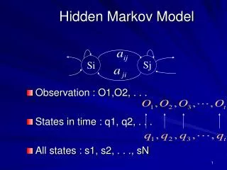
Hidden Markov model
E N D
Presentation Transcript
Hidden Markov model BioE 480 Sept 16, 2004
In general, we have Bayes theorem: P(X|Y) = P(Y|X)P(X)/P(Y) • Event X: the die is loaded, Event Y: 3 sixes. • Example: Assume we know that on average extracellular proteins have a slightly different a.a. composition than intracellular ones. Eg. More cysteines. How do we use this information to predict a new protein sequence x=x1x2…xn whether it is intracellular or extracellular. • We first split the training examples from Swiss-Prot into intracellular and extracellular proteins, leaving aside those unclassifiable. • We then estimate a set of frequencies for intraceullar proteins and a set of extracellular frequencies. • Also estimate the probability that any new sequence is extracelluar, pext and intracellular pint , called prior probabilites, because they are best guesses about a sequence before we actually see the sequence itself.
We now have: • Because we assume that every sequence must be either extracellular or intracelluar, we have: • By Bayes’ theorem, • This is the number we want: the posterior probability that a sequence is extracellular. • It is our best guess after we have seen the data. • More complicated: transmembrane proteins have both intra and extra cellular components.
Random Model R: For two sequences x and y, of lengths n and m. If xi is the i th symbol in x, and yi the i th symbol in y. Assume that letter a occurs independently with some frequency qa. • The probability of the two sequences x and y is just the product of the probabilities of each amino acid: P(x,y|R) = P qxiP qyi • An alternative model: Match Model M: Aligned pairs of residues occur with a joint probability Pab. Its value can be thought of as the probability that the resdiues a and b have each independently been derived from some unknown original residue c in their common ancester. • c might be the same as a and/or b. • The probability of the whole alignment is: P(x,y|M) = P pxiyi • The ratio of these two likelihoods is the odds ratio: P(x,y|M) / P(x,y|R) = P pxiyi / (P qxiP qyi )= P pxiyi / qxi qyi • To make this additive, we take the logarithm of this ratio, the log-odd ratio. S = S s(xi, yi), where s(a, b) = log (pab / qa qb ),
Here s(a, b) is the log likelihood ratio of the residue pair (a,b) occurring as an aligned pair, as opposed to an unaligned pair. A biologist may write down and ad hoc substitution matrix based on intuition, but it actually implies the “target frequencies” pab . Any substitution matrix is making a statement about the probability of observing ab pairs in real alignment. • How to develop an evolutionary model? • Parameterized by probability of residue A mutated to residue B: PAB • Statistical modeling: these parameters cannot be assigned, rather, they have to be estimated from data. • Suppose we know sequences s and s’ are related: find PAB that maximizes: • Maximum likelihood: maximize data likelihood under model. • Results:
Substitution matrix can be obtained when alignment of sequences are compiled. • Different matrix for different evolutionary time t : • How do we estimate it? • The probability of given a residue A and it is substituted by B within evolutionary distance t : • Ignore directionality of time: • Assume that the distribution of amino acid (a.a.) does not change during evolution: Can be estimated from: • relative frequency of pair (A,B) in the known alignment of s and s’, and • relative frequency qA of residue A. • Substitution matrix over a longer time scale:
Regular Expression • Widely used in many programs, especially those on Unix: awk, grep, sed, and perl. • Used for searching text files for a pattern. Eg. Search for all files that containing “C.elegans” or “Caenorhabditis elegans” with the regular expression: % grep “C[\.a-z]* elegans” * • This matches any line containing a C followed by any number of lower-case leters or “.”, then a space, and then “elegans”. • Another example, PROSITE. • Difficulty: need to be very broad and complex, because protein spelling is much more free than English spelling.
Example: ( use DNA because of the smaller number of letters than a.a.) ACA---ATG TCAACTATC ACAC--AGC AGA---ATC ACCG--ATC • A regular expression for this is: [AT][CG][AC][ACGT]*A[TG][GC] Problem: It does not distinguish: TGCT--AGG Highly implausible, exceptional character in each position ACAC--ATC Consensus sequence
Alternative: score sequences by how well they fit the alignment. • Eg. A proabability of 4/5=0.8 for A in the first position, 1/5=0.2 for a T; etc. • After the third position in the alignment, 3 out of 5 sequences have “insertions” of varying lengths, so we say the probability of making an insertion is 3/5 and thus 2/5 for not makng one. • A diagram: This is a hidden Markov model!
ACA---ATG TCAACTATC ACAC--AGC AGA---ATC ACCG--ATC ? A 0.8 C 0.0 G 0.0 T 0.2 A 0.0 C 0.8 G 0.2 T 0.0 A ? C ? G ? T ? A ? C ? G ? T ? A 1.0 C 0.0 G 0.0 T 0.0 A 0.0 C 0.0 G 0.2 T 0.8 A 0.0 C 0.8 G 0.2 T 0.2 ? ? ? ? 1.0 1.0 1.0
Hidden Markov Model • A box is called a “(Match) state”: • one state for each term in the regular expression. • Probabilities: counting in the multiple alignment how many times each event occurs. • “Insertion”: A state above the other states. • Probabilities of NTs: counting all occurrences of the four NTs in this region of the alignment: A 1/5; C 2/5; G 1/5, and T 1/5. • Probabilities of transitions: • After sequences 2, 3 and 5 have made one insertion each, there are two more (from sequence 2) • Total number of transitions back to the main line is 3: there are three sequences that have insertions. All will come back to the main states. • Therefore, probability of making a transition to the next state: 3/5 • Probability of making a transition to itself: 2/5 --- keep inserting.
Scoring Sequences • Consensus sequences: ACACATC. • Probability of the 1st A: 4/5. • This is multiplied by the probability of the transition from the first state to the second, which is 1. • …. • How do we score the exceptional sequence TGCT--AGG? • This is 2000 times smaller. • We can now get a score for each sequence to measure how well it fits the motif.
For the other four original sequences: • The probability depends very strongly on the length of the sequence. • Probability: Not a good number as score. • Use log-odds ratio: ln( observed/random), here the random model (null model) is that the sequences are random strings of NTs: • the probability of a sequence of length L is: 0.25 L
The log-odds score is: • Other null model: not 0.25, but background NT compositions. • When a sequence fits a HMM very well: high log-odds score • When it fits a null model better: negative score.
The second sequence has raw score as low as the exceptional score • because it has three inserts. • But the log-odds score is much higher than the exceptional seq. • Excellent discrimination. • But, high log-odds may not be a “hit”: there will always be random hits when searching a database. Need to look at E-value and P-value. • If the alignment had no gaps or insertions: • No insert state. • All probabilities associated with the arrows (the transition probabilities) = 1. Can all be ignored. • HMM works then exactly as a weight matrix of log-odds scores.
What is hidden • Come back to the occasional dishonest casino: they use a fair die most of the time, with a probability of 0.05 it switching to loaded die, and with a probability of 0.1 of switch back. • The switch between die is a Markov process (it only depends on the previous state). • The observation of the sequence of rolls is hidden Markov process because the casino wouldn’t tell you in which role they were using loaded die.
Profile HMMs • Profile HMMs: allows position-dependent gap penalties. • Obtained from a multiple alignment. • Can be used to search a database for other members of the family just like a standard profile. • Structure of the Model: • Main states (bottom): model the columns of the alignment, are the main states. • Probabilities are calculated by the frequency of the a.a. or NT. • Insert states (diamond): model highly variable regions in the alignment • Often the probabilities are a fixed distribution, eg, by composition
Delete states (circle): silent or null state. Do not match any residues, they are there so it is possible to jump over one or more columns: • For modeling when just a few of the sequences have a “-” at a position. • Example:
Insertion region (white): an alignment of this region is highly uncertain. • Shaded region: columns that correspond to main states in the HMM model. • Probabilities: For each non-insert column, we make a main state and set the probabilities equal to the amino acid frequencies. • Transition probabilities: count how many sequences use the various transitions, like before. • Delete states: Two transitions from a main state to a delete state, shown with dashed lines: • from “begin” to the first delete state • from main state 12 to delete state 13. • Both correspond to dashes in the alignment: • Only one sequence has gaps, the probability of these delete transitions is 1/30. • The 4th sequence continues deletion to the end: • Probability from delete 13 to 14 is 1, and from delete 14 to the end is also 1.
Pseudo-counts • Dangerous to estimate a probability distribution from just a few observed amino acids. • If there are two sequences, with Leu at a position: • P for Leu =1, but P = 0 for all other residues at this position • But we know that often Val substitutes Leu. • The probability of the whole sequence are easily become 0 if a single Leu is substituted by a Val. • Or , the log-odds is minus infinity. • How to avoid “over-fitting” (strong conclusions drawn from very little evidence)? • Use pseudocounts: • Pretend to have more counts than those from the data. • A. Add 1 to all the counts: • Leu: 3/23, other a.a.: 1/23
Adding 1 to all counts is as assuming a priori all a.a. are equally likely. • Another approach: use background composition as pseudocounts.