Hidden Markov Model
Hidden Markov Model. Ka-Lok Ng Dept. of Bioinformatics Asia University. 1. 2. 3. Hidden Markov Models and Gene Finding. A rabbit has three homes Three states 1, 2, 3 State transition such as 1 2, 2 1 … etc Discrete stochastic process


Hidden Markov Model
E N D
Presentation Transcript
Hidden Markov Model Ka-Lok Ng Dept. of Bioinformatics Asia University
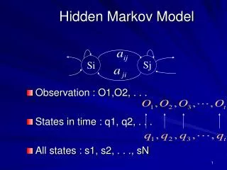
1 2 3 Hidden Markov Models and Gene Finding A rabbit has three homes Three states 1, 2, 3 State transition such as 1 2, 2 1 … etc Discrete stochastic process (x0, x1, ….xn) denotes the random sequence of the process where is the rabbit is located
Hidden Markov Models and Gene Finding • The occurrence of a future state in a Markov processdepends on the immediately preceding state and only on it. • The matrix P is called a homogeneous transition or stochastic matrix because all the transition probabilities pijare fixed and independent of time.
Hidden Markov Models and Gene Finding • A transition matrixP together with the initial probabilities associated with the states completely define a Markov chain. • One usually thinks of a Markov chain as describing the transitional behavior of a system over equal intervals. • Situations exist where the length of theinterval depends on the characteristics of the system and hence may not be equal. This case is referred to as imbedded Markov chains.
Bayes probability • Events A and B • Marginal probability, p(A), p(B) • Joint probability, p(A,B)=p(AB)=p(A∩B) • Conditional probability • p(B|A) = given the probability of A, what is the probability of B • p(A|B) = given the probability of B, what is the probability of A http://www3.nccu.edu.tw/~hsueh/statI/ch5.pdf
Bayes probability • General rule of multiplication • p(A∩B)=p(A)p(B|A) • = event A occurs *(after A occurs, then event B occurs) • =p(B)p(A|B) = event B occurs *(after B occurs, then event A occurs) • Joint = marginal * conditional • Conditional = Joint / marginal • P(B|A) = p(A∩B) / p(A) • How about P(A|B) ?
Bayes probability Given 10 films, 3 of them are defected. What is the probability two successive films are defective? 7 Good 3 Defects
Bayes probability Loyalty of managers to their employer.
Bayes probability Probability of new employee loyalty
Bayes probability Probability (over 10 year and loyal) = ? Probability (less than 1 year or loyal) = ?
Hidden Markov Models and Gene Finding Let (x0, x1, ….xn) denotes the random sequence of the process Joint probability is not easy to calculate. More easy withcalculatingconditional probability
Hidden Markov Models and Gene Finding HMMs – allow for local characteristics of molecular seqs. To be modeled and predicted within a rigorous statistical framework Allow the knowledge from prior investigations to be incorporated into analysis An example of the HMM Assume every nucleotide in a DNA seq. belongs to either a ‘normal’ region (N) or to a GC-rich region (R). Assume that the normal and GC-rich categories are not randomly interspersed with one another, but instead have a patchiness that tends to create GC-rich islands located within larger regions of normal sequence.
Hidden Markov Models and Gene Finding The states of the HMM – either N or R NNNNNNNNNRRRRRNNNNNNNNNNNNNNNNNRRRRRRRNNNN The two states emit nucleotides with their own characteristic frequencies. The word ‘hidden’ refers to the fact that the true states is unobserved, or hidden. TTACTTGACGCCAGAAATCTATATTTGGTAACCCGACGCTAA seq. 60% AT, 40% GC not too far from a random seq. If we focus on the red GC-rich regions 83% GC (10/12), compared to a GC frequency of 23% (7/30) in the other seq. HMMs – able to capture both the patchiness of the two classes and the different compositional frequencies within the categories.
Hidden Markov Models and Gene Finding HMMs applications Gene finding, motif identification, prediction of tRNA, protein domains In general, if we have seq. features that we can divide into spatially localized classes, with each class havingdistinct compositions HMMs are a good candidate for analyzing or finding new examples of the feature.
Hidden Markov Models and CG rich region Hidden Markov Models and Gene Finding • Training the HMM • The states of the HMM are the two categories, N or R. Transition probabilities govern the assignment of stated from one position to the next. In the current example, if the present state is N, the following position will be N with probability 0.9, and R with probability 0.1. The four nucleotides in a seq. will appear in each state in accordance to the corresponding emission probabilities. • The working of an HMM 2 steps • Assignment of the hidden states. • Emission of the observed nucleotides conditional on the hidden states N R
1 2 Hidden Markov Models and Gene Finding Consider the seq. TGCC arise from the set of hidden state NNNN. The probability of the observed seq. is a product of the appropriate emission probabilities: Pr(TGCC|NNNN) = 0.3*0.2*0.2*0.2 = 0.0024 where Pr(T|N) = conditional probability of observing a T at a site given that the hidden state is N. In general the probability is computed as the sum over all hidden states as:
Hidden Markov Models and Gene Finding The description of the hidden state of the first residue in a seq. introduces a technical detail beyond he scope of this discussion, so we simplify by assuming that the first position is a N state 2*2*2=8 possible hidden states
Hidden Markov Models and Gene Finding The most likely path is NNNN which is slightly higher than the path NRRR (0.00123). We can use the path that contributes the maximum probability as our best estimate of the unknown hidden states. If the fifth nucleotide in the series were a G or C, the path NRRRR would be more likely than NNNNN.
Hidden Markov Models and Gene Finding Hidden Markov Models and Gene Finding Figure on the right - Schematic of the hidden states included in an HMM Boxes = signal sensors for regulatory elements, coding region start sites, intron donor and acceptor sites, and translation stop sites Arrows = content sensors for intergenic regions, exons, and introns, Each of these regions emits nucleotides with frequencies characteristic of that region, with these frequencies being obtained by training the HMM on data sets of many known genes.
Figure. Predicting genes. Three different prediction methods (Ensembl, Fgenesh, and Genscan) were used on a region of chromosome 17 that includes the well-annotated GOSR2 gene. The black images below indicate the location of matching cDNA/EST sequences. Hidden Markov Models and Gene Finding