Download
1 / 38
380 likes | 550 Vues
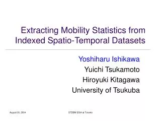
Extracting Mobility Statistics from Indexed Spatio-Temporal Datasets. Yoshiharu Ishikawa Yuichi Tsukamoto Hiroyuki Kitagawa University of Tsukuba. Outline. Background and objectives Markov transition probability Indexing method for moving trajectories Proposed methods naïve algorithm

E N D
Extracting Mobility Statistics from Indexed Spatio-Temporal Datasets Yoshiharu Ishikawa Yuichi Tsukamoto Hiroyuki Kitagawa University of Tsukuba STDBM 2004 at Toronto
Outline • Background and objectives • Markov transition probability • Indexing method for moving trajectories • Proposed methods • naïve algorithm • CSP-based algorithm • Experimental results • Conclusions
Background • Moving object databases • stores and manages information on a huge number of moving objects • supports queries on moving trajectories and/or moving status • Research issues • spatio-temporal indexes • extraction of statistics (e.g., selectivities) • Statics in spatio-temporal databases • used for query optimization • also useful in mobility analysis
Our Approach • Objective: extracting mobility statistics from spatio-temporal databases • Target: trajectory data indexed using R-trees • Statistics to be extracted:Markov transition probability • target space is decomposed in cells • estimating transition probabilities between cells using the indexed trajectory data • Features • search problem is formalized as constraint satisfaction problem (CSP) • efficient processing usingR-trees
Outline • Background and objectives • Markov transition probability • Indexing method for moving trajectories • Proposed methods • naïve algorithm • CSP-based algorithm • Experimental results • Conclusions
A A t =τ t =τ+1 Markov Transition Probability (1) • Assumption: target space is decomposed in cells • Example 1: What is the estimated probability that an object currently in cell c0moves in cell c1in a unit time later? • First-orderMarkov transition probability Pr(c1|c0) c0 c1
A A A c1 c2 t =τ t =τ+1 t =τ+2 Markov Transition Probability (2) • Example 2: What is the probability that an object which moves from c0to cell c1in a unit time moves to cell c2in the next unit time? • Second-order transition probability Pr(c2|c0, c1) • Extension toorder-n Markov transitionprobability Pr(cn|c0, …, cn-1) is easy c0
Markov Transition Probability • Conventional technique in traffic data analysis • Upton & Fingleton, 1989 [13] • Special kind of association rules • probability corresponds to the confidence factor • difference: existence of order • Usage • trajectory estimation • estimates where a moving object moves to in the next period • simulation of movement status • given status of moving objects at t = , we can estimate the change of the status at t = + 1, + 2, …
Assumptions • Movement patterns obeys stationaryprocess • movement tendency does not change as time passes • Cell decomposition • each cell is a rectangle • cell size is arbitrary: non-uniform decomposition is allowed • cell decomposition can be specified dynamically • Unit time length • unit time can be specified as arbitrary length (e.g., one minuite, 10 minuites, …) • but a unit time length should be a multiple of sampling time length
Formalization of Probability (1) • Target data: trajectory data fromt = 0 to t = T • Definition of first-order Markov transition probability • objs(ci, t): set of objects which were in cell ci at t • denominator: no. of objects which were in cell c0 at arbitrary t (0 ≤t ≤T 1) • numerator: no. of objects each of which contained in denominator and moved cell c1 at t + 1
Formalization of Probability (2) • Definition of order-n Markov Transition Probability • denominator: no. of objects each of which was in cell c0 at t (0 ≤ t ≤T 1), in cell c1 at t+ 1, …, and in cell cn 1 at t+ n 1 • numerator: no. of objects each of which is contained in Dominator and moved cell cn at t + n
Generalized Transition Probability Estimation Problem (1) • Derives transition probability according to the specified cell sets at once • Given n + 1 cell sets • for each of arbitrary cell combinations • outputPr(cn|c0,…,cn-1)
c0 c1 c2 c3 Generalized Transition Probability Estimation Problem (2) • Example: Given C0 = {c0, c1}, C1 = {c1, c2}, C2 = {c1, c2, c3}, estimate second-order probabilities • Algorithm outputs 12 probabilities Pr(c1|c0, c1), Pr(c2|c0, c1), …, Pr(c3|c1, c2)
Outline • Background and objectives • Markov transition probability • Indexing method for moving trajectories • Proposed methods • naïve algorithm • CSP-based algorithm • Experimental results • Conclusions
Indexing Methods for Trajectories • R-tree-based approach is assumed • Point-based representation: trajectories is represented as a set of points • (d+1)-dimension R-tree is used (e.g., 3D R-tree) • incorporating temporal dimension
x x root b 1 5 6 3 a 4 c 2 root 0 1 2 3 4 5 6 7 8 (=T) 0 1 2 3 4 5 6 7 8 (=T) a b c 1 2 3 4 5 6 (d +1)-D R-tree-based Representation B A Sampling-based representation
Outline • Background and objectives • Markov transition probability • Indexing method for moving trajectory data • Proposed methods • naïve algorithm • CSP-based algorithm • Experimental results • Conclusions
Naïve Algorithm (1) • Based on the definition of the Markov transition probability • Example: Estimating Pr(c2|c0, c1) • Determine objs(c0, ) and objs(c1, + 1) using the R-tree • objs(ci, t): the set of objects which were in cellciat time t • Take intersection of two sets; the cardinality of the intersection is added to Scount • If the intersection is not empty objs(c2, + 2) is determined using the R-tree • Take intersection of objs(c0, ), objs(c1, + 1) , objs(c2, + 2);the cardinality of the result is added toQcount • This process is repeated for each (0 ≤≤T – n) • CalculatePr(c2|c0, c1) based on Scount, Qcount • No. of search on R-tree is proportional to T
cell c0 cell c1 Output = Qcount Scount x Qcount += 1 cell c2 0 1 2 3 4 5 6 7 8 (=T) No. of search on R-tree is proportional to T Scount += 1 Scount += 1 Naïve Algorithm (2) Example: estimation of
Outline • Background and objectives • Markov transition probability • Indexing method for moving trajectories • Proposed methods • naïve algorithm • CSP-based algorithm • Experimental results • Conclusions
Basic Idea (1) • Estimation of Pr(cn|c0, …, cn-1) based on three steps: • Count the no. of objects which were in c0, …, cn-1 at each unit time using an R-tree • Count the no. of objects which were in c0, …, cnat each unit time using an R-tree • Compute Pr(cn|c0, …, cn-1) by [result of step 2] / [result of step 1] • Benefits • step 1 & 2 can be processed using the same algorithm • algorithm for step 1 is given by setting n → n – 1 • requires only two searches on R-tree
Basic Idea (2) Example: estimation of Pr(c2|c0, c1) x Step 1: count objects which moved from c0 toc1within a unit time cell c2 Step 2: count objects that moved as c0 , c1, c2 at each unit time cell c1 Step 3: compute probability cell c0 Qcount = 1 Pr(c2|c0, c1) = ――――― Scount = 2 0 1 2 3 4 5 6 7 8 (= T)
Counting Using R-tree (1) • How can we compute no. of objects which were in c0, …, cnat each unit time? • Idea: the problem is formalized as a constraint satisfaction problem (CSP) • An object satisfying the constraint fulfills the following constraints for some • it was in cellc0at t = • it was in cellc1at t = + 1 • … • it was in cellcnat t = + n • Search objects that satisfy all n + 1 constraints
Counting Using R-tree (2) • Effective use of R-tree is necessary • We extend the CSP solution search method using R-trees(Papadias et al, VLDB’98) [7] • considers spatial constraints • Example: find all spatial objects x, y, z that satisfy overlap(x, y) and north(y, z) • search CSP solutions from the root to leaves • Use of pruning and backtracks • Reduce search space using constraints • enumerates all solutions with one R-tree access
x 0 1 2 3 4 5 6 7 8 (=T) Example of Counting (1) root ForC0 = {c1}, C1 = {c1, c2}, C2={c2}, derive probabilities for(C0, C1, C2) b 1 5 6 3 • Derive two probabilities at once • Pr(c2|c1, c1): the probability that an objectwhich have moved as c1c1 next moves to c2 • Pr(c2|c1, c2) c2 a 4 c 2 c1
x 0 1 2 3 4 5 6 7 8 (=T) Example of Counting (2) root R-tree b root 1 5 6 3 c2 a a b c 4 c 2 c1 1 2 3 4 5 6
x c b a 0 1 2 3 4 5 6 7 8 (=T) Pruning Method (1) Pruning condition 1: Movement between two R-tree nodes which do not temporary consecutive is impossible Candidates can be deleted Example: • movement such as ab and bc are allowed • movement ac is impossible
x 0 1 2 3 4 5 6 7 8 (=T) Pruning Method (2) Pruning condition 2: Trajectory is not contained in the target cell Example: When we are counting for c1 c1, we should consider only nodesthat overlaps with c1 cellc1
x 1 2 0 1 2 3 4 5 6 7 8 (=T) Pruning Method (3) Pruning condition 3: If [max distance an objectcan move] < [distance betweenMBRs] then an object cannotmove from a node to next node distance between MBRs
Query Processing Example x treelevel = 2 root root root cell c2 cell c2 cell c2 a c b cell c1 cell c1 cell c1 t 1 2 There is no objects that moved as c1 c1 c2 c1 c2 c2 backtrack An object that moved as c1 c1 c2 is found and counted Targets: c1 c1 c2 c1 c2 c2 pruning pruning treelevel = 1 pruning tree level =0
Outline • Background and objectives • Markov transition probability • Indexing method for moving trajectory data • Proposed methods • Naïve algorithm • CSP-based algorithm • Experimental results • Conclusions
Dataset (1) • Generated using the moving object simulator made by Brinkoff [1] • Simulates car movement situation on actual city road network • Oldenburg city, Germany (about 2.5km x 2.8km) • no. of initial moving objects: 5 • 5 objects are created in a minute • on average 100 objects are moving in the map at a time • data is generated for T = 1000 minutes • 120K points are stored in 3-D R-tree
c0 c3 c6 c1 c4 c7 c2 c5 c8 0 0.183 0.04 0.081 0.348 0.10 0.08 0.01 0.02 Dataset (2) Example for estimating using 3 x 3 cells
Experimental Result (1) • Map is decomposed into 30 x 30 cells • First-order Markov transition probabilities • Randomly 3 x 3 cells are selected
Experimental Result (2) • Estimation of second-order transition probabilities • Other parameters are same to the former case
Experimental Result (3) • Estimation of third-order transition probabilities • Other parameters are similar to the former case
Experimental Result (4) • The case when CSP-based approach is not effective • Target space is decomposed into 20 x 20 cells • Estimation of second-order transition probabilities Since cell decomposition is coarse, the pruning cannot reduce candidates
Conclusions and Future Work • Conclusions • mobility statistics based on Markov transition probability • proposals of two algorithms • naïve approach • CSP-based approach • CSP-based approach effectively utilizes R-tree structure • Future Work • adaptive cell decompositions • extension to non-stationary Markov transitions