Understanding Convolution in Computer Vision
Learn about the fundamental operation of computer vision - Convolution. Discover how it works, its mathematical definitions, fascinating kernels, edge handling techniques, interesting applications, and the significance of normalization. Dive into specific examples like Gaussian Filters and Sobel Edge Detection.

Understanding Convolution in Computer Vision
E N D
Presentation Transcript
Convolution Operators CSC508
Convolution • Arguably the most fundamental operation of computer vision • It’s a neighborhood operator • Similar to the median and outlier processes we discussed last week • Utilizes a pattern of weights defined over the neighborhood • Also known as • A filter • A kernel CSC508
Convolution • Mathematically defined as The resultant image The input image neighborhood The kernel or filter u x v The size of the kernel • H is convolved with F yielding R CSC508
Convolution • But what does it really mean? • It’s a “multiply/accumulate” operation j i Kernel Image CSC508
Consider 1-Dimensional Input CSC508
A 1-Dimensional Kernel CSC508
Convolution in 1-Dimension CSC508
1-Dimension Output CSC508
Convolution • We “slide” the kernel over the entire image • In two dimensions we just slide the kernel top to bottom and left to right • Eventually it gets centered over every pixel • Note, we typically do this operation so that all pixels are handled in parallel (simultaneously) • It’s a fairly “expensive” operation • What about the edges of the image? • Various techniques can be employed CSC508
Convolution at the Edges • Just ignore the edges • Initialize the resultant image to 0 (or something else) • Use only the parts of the kernel that are within the image • Enlarge the input image on all sides by reflection CSC508
Enlarging by Reflection Assume a 3x3 kernel Original image A larger kernel requires additional reflection CSC508
Why Reflect? • Why not just pad with 0 (or some other value)? • We’ll see later when we look at edge detection CSC508
Some Interesting Kernels • Neighborhood averaging • A simple blurring function • Note that the results of the convolution may go out of range • Solution is to normalize the kernel • Various techniques • Divide each kernel by the sum of all values • Divide the result by the sum of all values CSC508
Neighborhood Averaging CSC508
Emboss Not really useful for computer vision but interesting none the less Why don’t we need to normalize this kernel? But, we do need to make sure the output does not go below 0 (since a kernel value is negative) Some Interesting Kernels CSC508
Emboss CSC508
Laplacian A simple gradient detection mask What is the range of the result? [-1020..1020] Need to do something about this (clamp or scale) Some Interesting Kernels CSC508
Laplacian CSC508
Some Interesting Kernels • You can set the kernel weights to any values you want • Anything that will give you the desired effect • Selecting “meaningful” weights is an art CSC508
Gaussian Kernel (Filter) • The Gaussian filter is a smoothing or blurring filter • Width is the number of pixels covered by the filter • Sigma is the standard deviation of the Gaussian curve in pixels CSC508
Coding the Gaussian • Use odd number of rows and columns in the kernel (e.g. 3x3, 5x5, 7x7…) • Loop over every location in the kernel matrix • Translate integer indices from [0..width-1] to floating point [–width/2..+width/2] • This makes the floating point coordinate of the central value (0.0, 0.0) • Perform the calculation given with the translated loop indices as the x and y values • When done, normalize the kernel coefficients by dividing each coefficient by the sum of all coefficients CSC508
Gaussian Filter • Sigma 1.0, Filter Width 7 CSC508
Gaussian Filter • Sigma 1.6, Filter Width 7 CSC508
Gaussian Filter • Sigma 1.6, Filter Width 15 CSC508
Gaussian is Separable • Two 1D Gaussians produces the same results a one 2D Gaussian • First convolve the original image horizontally • Then convolve the horizontal results vertically • This speeds things up dramatically • Reduces the total number of multiplies and additions CSC508
Gaussian Filter – 1D CSC508
Gaussian Filter – 1D • Sigma 1.6, Filter Width 15 CSC508
Gaussian Filter • Why would we want to blur an image? • It will help us to extract gradient features (edges) CSC508
Edge Detection • What is an edge? • An intensity gradient • That is, a change of intensity within a localized region of the image (a neighborhood) The edge CSC508
Edge Detection • Is there an edge here? • There is definitely a gradient but no edge • At least not over a small neighborhood CSC508
Edge Detection • Edges are described by magnitude which is related to the intensity on either side of the edge Weaker edge Strong edge CSC508
Edge Detection • Edges are described by orientation (direction) • Orientation is determined by the angle of the gradient and the intensity on either side of the gradient CSC508
Edge Detection • Various techniques • Differential operator • Sobel • Templates • Nevatia-Babu • Procedural • Marr-Hildreth (Laplacian-Gaussian) • Canny CSC508
Sobel Edge Operator • Starts with two convolution kernels • Perform two convolutions on the original image resulting in two intermediate images CSC508
Sobel Edge Operator • From the two convolved images you can now compute edge magnitude and direction • The magnitude will have to be scaled to 0..255 • Unscaled values will be both + and - • The direction is typically scaled to a small number of bins • i.e. 0..8 or 0..16 CSC508
If we were to zoom in on the corners we’d see other edge orientations present This edge is not missing, it’s just the same color as the background Sobel Edge Operator Encoded Direction Magnitude Input CSC508
Nevatia-Babu Template Operator • Six edge-oriented convolution kernels (templates) 0-deg 30-deg 60-deg 90-deg 120-deg 150-deg CSC508
Nevatia-Babu Template Operator • Convolve each image pixel with all six kernels • Select the mask that produces the maximum output • Assign the magnitude to the output of the maximal mask • Assign the direction to the orientation of the maximal mask • Direction is further modified by the sign of the maximal mask • As you might imagine, this is a very time consuming operation CSC508
Things To Do • Programming homework assignment • Gaussian Convolution • Reflect the edges of the image • Implement as both a 2D convolution and 2 1D convolutions • “prove” that they are equivalent through code demonstrations • Sobel Edge Operator • You may write in any programming language you choose • Deliverables: • Zipped images in email • Email the source code to reinhart@clunet.edu with the subject line CSC508 PROGRAM 2 • Due beginning of class in two weeks • (late assignments will be penalized 10%) • I will post test images • Reading for Next Week • Still in chapter 8 • We’ll talk about • Non-maximal edge suppression • Edge following • Hysteresis • We’ll experiment with two edge detection algorithms • Marr-Hildreth (Laplacian-Gaussian/Difference of Gaussians) • Canny (Differential) CSC508