PARALLELIZED CONVOLUTION
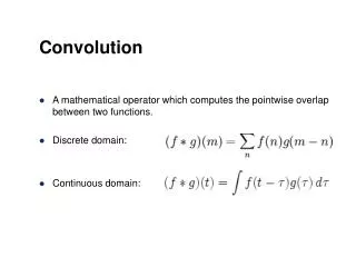
PARALLELIZED CONVOLUTION. Convolution. Convolution is a mathematical operation on two functions A function derived from two given functions by integration that expresses how the shape of one is modified by the other. The Mathematical expression for basic two dimensional convolution is.

PARALLELIZED CONVOLUTION
E N D
Presentation Transcript
Convolution • Convolution is a mathematical operation on two functions • A function derived from two given functions by integration that expresses how the shape of one is modified by the other. • The Mathematical expression for basic two dimensional convolution is
Applications • Image Processing • Electrical Engineering (Communication signal processing) • Statistics • Differential equations
Sequential solution • The kernel matrix is padded over the input matrix and the overlapping pixels are computed and this operation is continued for all the pixels of input matrix. • The complexity is similar to matrix multiplication where the computation involves huge no of multiplications and additions.
Parallel solution • Input Matrix is stored in a single node • Kernel matrix is broadcasted to all the other processors • Input Matrix node distributes chunks of input matrix to all the other processors • All the processors sends the partially computed result to a single final node • Because of independent convolutions, distributed parallelism can be implemented
The Input size • 1024 x 1024 image – input • 90 x 90 kernel
Choosing optimum N from the graph? xy=constant x+y=minimum xycost 1 64 64 2 32 64 8+8=16 - which is the minimum among 4 16 64 all x+y combinations. so choosing N (no 8 8 64 of processors) at this point will give fairly 16 4 64 best cost for a given input 32 2 64 64 1 64
Optimum N? • The optimum no of nodes for the approximate no of multiplications can be calculated. • example : 1024 x 1024 image – input 90 x 90 kernel - 1024 x 1024 x 90 x 90 = ~ 8 billionoperations
Difficulties • Communication overhead • Large no of multiplications - (~8 billion Multiplications and additions) for 90 x 90 kernel - (~6.5 billion Multiplications and additions) for 80 x 80 kernel • Filtering the input matrix
References • www.scribd.com/doc/58013724/10-MPI-programmes • http://heather.cs.ucdavis.edu/~matloff/mpi.html • Miller, Russ, and Laurence Boxer. Algorithms, sequential & parallel: A unified approach.