Understanding Convolution and Correlation in Image Processing
Learn about convolution, correlation, 1D continuous convolution, convolution with an impulse, efficient computation, discrete convolution, and 2D convolution, with examples and important observations.


Understanding Convolution and Correlation in Image Processing
E N D
Presentation Transcript
Convolution CS474/674 – Prof. Bebis Section 3.4, 4.2
Output Image Correlation - Review K x K
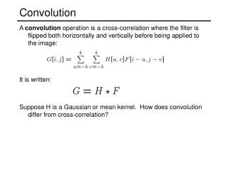
Convolution – Review (cont’d) • Same as correlation except that the mask is flipped both horizontally and vertically. • Note that if w(x,y) is symmetric, that is w(x,y)=w(-x,-y), then convolution is equivalent to correlation!
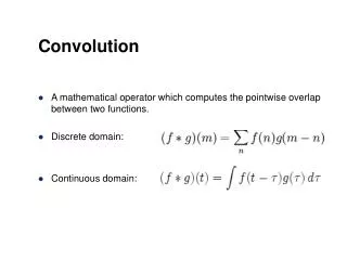
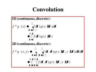
1D Continuous Convolution - Definition • Convolution is defined as follows: • Convolution is commutative
Example 2 • Suppose we want to compute the convolution of the following two functions:
Example 2 (cont’d) Step 3:
Important Observations • The extent of f(x) * g(x) is equal to the extent of f(x) plus the extent of g(x) • For every x, the limits of the integral are determined as follows: • Lower limit: MAX (left limit of f(x), left limit of g(x-a)) • Upper limit: MIN (right limit of f(x), right limit of g(x-a))
Example 3 α α
Convolution Theorem • Convolution in the spatial domain is equivalent to multiplication in the frequency domain. • Multiplication in the spatial domain is equivalent to convolution in the frequency domain. f(x) F(u) g(x) G(u)
Efficient computation of (f * g) • 1. Compute and • 2. Multiply them: • 3. Compute the inverse FT: (i.e., complex multiplication)
Discrete Convolution • Replace integral with summation • Integration variable becomes an index. • Displacements take place in discrete increments
Discrete Convolution (cont’d) 3 samples 5 samples g - 1)
Convolution Theorem in Discrete Case • Input sequences: • Length of output sequence: • Extended input sequences (i.e., pad with zeroes)
Convolution Theorem in Discrete Case (cont’d) • When dealing with discrete sequences, the convolution theorem holds true for the extended sequences only!! In general, we can choose
Why? continuous case discrete case The convolution of discrete sequences is a periodic function (with period M) since the DFT is periodic
Why? (cont’d) Α+Β+1 Α+Β+1 If M<A+B-1, the periods will overlap If M>=A+B-1, the periods will not overlap
2D Convolution • Definition • 2D convolution theorem
Discrete 2D convolution • Suppose f(x,y) is A x B and g(x,y) is C x D • The size of f(x,y) * g(x,y) would be N x M where N=A+C-1 and M=B+D-1 • Form extended images (i.e., pad with zeroes):
Discrete 2D convolution (cont’d) • The convolution theorem holds true for the extended images only.