Download
1 / 21
210 likes | 380 Vues
Improving Understanding of Global and Regional Carbon Dioxide Flux Variability through Assimilation of in Situ and Remote Sensing Data in a Geostatistical Framework. Kim Mueller 1 Sharon Gourdji 1 Anna M. Michalak 1,2 1 Department of Civil and Environmental Engineering

E N D
Improving Understanding of Global and Regional Carbon Dioxide Flux Variability through Assimilation of in Situ and Remote Sensing Data in a Geostatistical Framework Kim Mueller1 Sharon Gourdji1 Anna M. Michalak1,2 1Department of Civil and Environmental Engineering 2Department of Atmospheric, Oceanic and Space Sciences The University of Michigan
Synthesis Bayesian Inversion Prior flux estimates (sp) BiosphericModel CO2Observations (y) AuxiliaryVariables Inversion Flux estimates and covarianceŝ, Vŝ TransportModel Sensitivity of observations to fluxes (H) Meteorological Fields Residual covariancestructure (Q, R) Slide from Anna Michalak
Key Questions • Is there another inversion approach available to estimate: • Spatial and temporal autocorrelation structure of fluxes and/or flux residuals? • Sources and sinks of CO2 without relying on prior estimates? • Significance of available auxiliary data? • Relationship between auxiliary data and flux distribution? • Realistic grid-scale flux variability
Geostatistical Approach to Inverse Modeling • Geostatistical inverse modeling objective function: • H = transport information, s = unknown fluxes, y = CO2 measurements • X and define the model of the trend • R = model data mismatch covariance • Q = spatio-temporal covariance matrix for the flux deviations from the trend Deterministic component Stochastic component
Global Gridscale CO2 Flux Estimation • Estimate monthly CO2 fluxes (ŝ) and their uncertainty on 3.75° x 5° global grid from 1997 to 2001 in a geostatistical inverse modeling framework using: • CO2 flask data from NOAA-ESRL network (y) • TM3 (atmospheric transport model) (H) • Assume spatial correlation but no temporal correlation a priori(Q) • Three models of trend flux (Xβ) considered: • Simple monthly land and ocean constants • Terrestrial latitudinal flux gradient and ocean constants • Terrestrial gradient, ocean constants and auxiliary variables
Transcom Regions TransCom, Gurney et al. 2003
Regional comparison of seasonal cycle GtC/yr GtC/yr
Regional comparison of inter annual variability GtC/yr GtC/yr
Key Questions • Is there another inversion approach available to estimate: • Spatial and temporal autocorrelation structure of fluxes and/or flux residuals? • Sources and sinks of CO2 without relying on prior estimates? • Significance of available auxiliary data? • Relationship between auxiliary data and flux distribution? • Realistic grid-scale flux variability …. Sharon
Key Questions • Is there another inversion approach available to estimate: • Spatial and temporal autocorrelation structure of fluxes and/or flux residuals? • Sources and sinks of CO2 without relying on prior estimates? • Significance of available auxiliary data? • Relationship between auxiliary data and flux distribution? • Realistic grid-scale flux variability
Sample Auxiliary Data Gourdji et al. (in prep.)
Variance-Ratio Test and Auxiliary Variables Variance-Ratio Test uses atmospheric data to assess significant improvement in fit of more complex trend Physical understanding combined with results of VRT to choose final set of auxiliary variables: % Ag LAI SST % Forest fPAR dSSt/dt % Shrub NDVI Palmer Drought Index % Grass Precipitation GDP Density Land Air Temp. Population Density Variance-Ratio Test uses atmospheric data to assess significant improvement in fit of more complex trend Physical understanding combined with results of VRT to choose final set of auxiliary variables: % AgLAISST % ForestfPARdSSt/dt % ShrubNDVI Palmer Drought Index % Grass PrecipitationGDP Density Land Air Temp.Population Density ˆ • Three models of trend flux (Xβ) considered: • Monthly land and ocean constants (simple) • Terrestrial latitudinal flux gradient and ocean constants (modified) • Latitudinal gradient, ocean constants and auxiliary variables (variable)
Building up the best estimate in January 2000 ˆ Deterministic component Stochastic component Gourdji et al. (in prep.)
Uncertainty Reduction from Simple to Variable Trend % Gourdji et al. (in prep.)
Regional comparison of seasonal cycle Gourdji et al. (in prep.)
Comparison of annual average non-fossil fuel flux Gourdji et al. (in prep.)
Conclusions Atmospheric data information and geostatistical approach can: Quantify model-data mismatch and flux covariance structure Identify significant auxiliary environmental variables and estimate their relationship with flux Constrain continental-scale fluxes independently of biospheric model and oceanic exchange estimates Uncertainties at grid scale are high, but uncertainties of continental and global estimates are comparable to synthesis Bayesian studies Upscaling fluxes a posteriori minimizes the risk of aggregation errors associated with inversions that estimate fluxes directly at large scale Auxiliary data inform grid-scale flux variability; seasonal cycle at larger scales is consistent across models Use of auxiliary variables within a geostatistical framework can be used to derive process-based understanding directly from an inverse model
North American CO2 Flux Estimation • Estimate North American CO2 fluxes at 1°x1° resolution & daily/weekly/monthly timescales using: • CO2 concentrations from 3 tall towers in Wisconsin (Park Falls), Maine (Argyle) and Texas (Moody) • STILT – Lagrangian atmospheric transport model • Auxiliary remote-sensing and in situ environmental data Pseudodata and recovered fluxes (Source: Adam Hirsch, NOAA-ESRL)
Acknowledgements Collaborators: Advisor: Anna Michalak Research group: Alanood Alkhaled, Abhishek Chatterjee, Sharon Gourdji, Charles Humphriss, Meng Ying Li, Miranda Malkin, Kim Mueller, Shahar Shlomi, and Yuntao Zhou Data providers: NOAA-ESRL cooperative air sampling network Christian Rödenbeck, MPIB Kevin Schaefer, NSIDC Funding sources:
QUESTIONS? kimlm@umich.edu & sgourdji@umich.edu