Shortest Path Problem

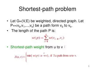
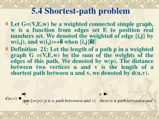
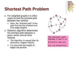
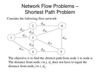
1. Shortest Path Problem • For weighted graphs it is often useful to find the shortest path between two vertices • Here, the “shortest path” is the path that has the smallest sum of its edge weights • Dijkstra’s algorithm determines the shortest path between a given vertex and all other vertices • The algorithm is named after its discoverer, Edgser Dijkstra • it is assumed that weight of edges are positive A 1 4 B C 5 3 2 E 1 5 D 8 1 F 2 G The shortest path between B and G is: B–D–E–F–G and not B–G (or B–A–E–F–G)

2. Dijkstra’s Algorithm • Finds the shortest path to all nodes from the start node • Performs a modified BFS that accounts for cost of vertices • The cost of a vertex (to reach a start vertex) is weight of the shortest path from the start node to the vertex using only the vertices which are already visited (except for the last one) • Selects the node with the least cost from unvisited vertices • In an unweighted graph (weight of each edge is 1) this reduces to a BFS • To be able to quickly find an unvisited vertex with the smallest cost, we will use a priority queue (highest priority = smallest cost) • When we visit a vertex and remove it from the queue, we might need to update the cost of some vertices (neighbors of the vertex) in queue (decrease it) • The shortest path to any node can be found by backtracking in the results array (the results array contains, for each node, the minumum cost and a “parent” node from which one can get to this node achieving the minimum cost)

3. Dijkstra’s Algorithm – Initialization • Initialization – insert all vertices in a priority queue (PQ) • Set the cost of the start vertex to zero • Set the costs of all other vertices to infinity and their parent vertices to the start node • Note that because the cost to reach the start vertex is zero it will be at the head of the PQ • Special requirement on priority queue PQ: • we can use min-heap • a cost of an item (vertex) can decrease, and in such case we need to bubble-up the item (in time O(log n)) • another complication is that we need to locate the item in the queue which cost has changed, but we know its value (vertex number) but not its location in the queue – therefore, we need to keep reversed index array mapping vertices to positions in the heap

4. Priority Queue Interface publicclass Vertex { privateint number; // vertex number: 0..|V|-1 privatedouble cost; privateint parent; // constructors, accessors, mutators } publicinterface VertexPQInterface { // using min-heap // costs of the vertices are used as priorities (keys) publicboolean isEmpty(); publicvoid insert(Vertex v); // O(log n) public Vertex extractMin(); // O(log n) // remove the vertex with smallest cost publicint find(int vertexNumber); // O(1) // return index of vertex v publicvoid decreaseCost(int i, double newCost); // O(log n) // decrease the cost of vertex in position i of the heap }

5. Dijkstra’s Algorithm – Main Loop • Until PQ is empty • Remove the vertex with the least cost and insert it in a results array, make that the current vertex (cv) [it can be proved that the cost of this vertex is optimal] • Search the adjacency list of cv for neighbors which are still in PQ • For each such vertex, v, perform the following comparison • If cost[cv] + weight(cv,v) < cost[v] change v’s cost recorded in the PQ to cost[cv] + weight(cv,v) and change v’s parent vertex to cv • Repeat with the next vertex at the head of PQ

6. Dijkstra Algorithm Outline publicclass Dijkstra { Vertex results[]; Dijkstra(WeightedGraphList G,int start) { // create a VertexPQ and insert all vertices // loop: // extract min-cost vertex and put it to results // update costs of neighbors in PQ } double costTo(int v) { return results[v].getCost(); } void printPathTo(int v); }

7. Dijkstra’s Algorithm – Final Stage • When the priority queue is empty the results array contains all of the shortest paths from the start vertex • Note that a vertex’s cost in the results array represents the total cost of the shortest path from the start to that vertex • To find the shortest path to a vertex from start vertex look up the goal vertex in the results array • The vertex’s parent vertex represents the previous vertex in the path • A complete path can be found by backtracking through all of the parent vertices until the start vertex is reached

8. Find the Shortest Path … • The shaded squares are inaccessible • Square 13 is the start square • Moves can be made vertically or horizontally (but not diagonally) one square at a time • The cost to reach an adjacent square is indicated by the wall thickness:

9. 02 04 05 3 3 2 1 06 07 08 09 10 11 2 1 3 4 5 1 1 2 12 13 14 1 2 1 1 2 18 19 20 22 23 2 2 5 2 3 2 26 27 28 29 2 3 5 4 5 5 1 32 33 34 35 2 1 1 Graph Representation • Only vertices that can be reached are to be represented • Graph is undirected • As the cost to move from one square to another differs, the graph is weighted • The graph is fairly sparse, suggesting that the edges should be stored in an adjacency list

10. 02 04 05 3 3 2 1 06 07 08 09 10 11 2 1 3 4 5 1 1 2 12 13 14 1 2 1 1 2 18 19 20 22 23 2 2 5 2 3 2 26 27 28 29 2 3 5 4 5 5 1 32 33 34 35 2 1 1 Graph Representation • Only vertices that can be reached are to be represented • Graph is undirected • As the cost to move from one square to another differs, the graph is weighted • The graph is fairly sparse, suggesting that the edges should be stored in an adjacency list

11. 02 04 05 3 3 2 1 06 07 08 09 10 11 2 1 3 4 5 1 1 2 12 13 14 1 2 1 1 2 18 19 20 22 23 2 2 5 2 3 2 26 27 28 29 2 3 5 4 5 5 1 32 33 34 35 2 1 1 Dijkstra’s Algorithm Start    • The cost to reach each vertex from the start (st) is set to infinity • For vertex v let's call this cost c[st][v] • All nodes are entered in a priority queue, in cost priority • The cost to reach the start node is set to 0, and the priority queue is updated • The results list is shown in the sidebar        0              

12. 02 04 05 06 07 08 09 10 11 12 13 14 18 19 20 22 23 26 27 28 29 32 33 34 35 Dijkstra’s Algorithm Demonstration  5   vertex, cost, parent 3 13, 0, 13 07, 1, 13 2 3   1 3 2   5 2  1  12, 1, 13 19, 1, 13 2 1 3 4 5 14, 2, 13 06, 2, 12 1 1 2 1  0  2 08, 2, 07 18, 2, 12 1 2 remove start from PQ 1  2 1 1  2  3   2 2 5 update cost to adjacent vertex, v, via removed vertex, u, if: c[u][v] + c[st][u] < c[st][v] 2   3  2  2 3 5 4 5 5 1     2 1 1

13. 02 04 05 06 07 08 09 10 11 12 13 14 18 19 20 22 23 26 27 28 29 32 33 34 35 Dijkstra’s Algorithm Demonstration vertex, cost, parent 5 11  14  3 13, 0, 13 10, 9, 09 07, 1, 13 32, 9, 26 2 1 3 2 5 2  9 1 14  12, 1, 13 28, 10, 27 19, 1, 13 04, 11, 10 2 1 3 4 5 14, 2, 13 33, 11, 32 06, 2, 12 34, 12, 33 1 1 2 1 0 2 08, 2, 07 22, 13, 28 18, 2, 12 35, 13, 34 1 2 20, 3, 19 05, 14, 04 02, 5, 08 11, 14, 10 1 2 1 1 2 3 13  18 16  09, 5, 08 29, 14, 35 26, 5, 20 23, 16, 29 2 2 5 27, 7, 26 2  5 7  3 10  2 15 14  2 3 5 4 5 5 1 9  11 12  12 15  13  2 1 1

14. Retrieving the Shortest Path • Having completed the array of results paths from the start vertex can now be retrieved • This is done by looking up the end vertex (the vertex to which one is trying to find a path) and backtracking through the parent vertices to the start • For example to find a path to vertex 23 backtrack through: • 29, 35, 34, 33, 32, 26, 20, 19, 13 • Note: there should be some efficient way to search the results array for a vertex vertex, cost, parent 13, 0, 13 10, 9, 09 07, 1, 13 32, 9, 26 12, 1, 13 28, 10, 27 19, 1, 13 04, 11, 10 14, 2, 13 33, 11, 32 06, 2, 12 34, 12, 33 08, 2, 07 22, 13, 28 18, 2, 12 35, 13, 34 20, 3, 19 05, 14, 04 02, 5, 08 11, 14, 10 09, 5, 08 29, 14, 35 26, 5, 20 23, 16, 29 27, 7, 26

15. 06 07 08 12 14 18 Shortest Path from Vertex 13 to 23 5 11 14 02 04 05 3 vertex, cost, parent 2 1 3 2 5 2 9 1 14 13, 0, 13 10, 9, 09 09 10 11 07, 1, 13 32, 9, 26 2 1 3 4 5 12, 1, 13 28, 10, 27 1 1 2 1 0 2 19, 1, 13 04, 11, 10 14, 2, 13 33, 11, 32 13 1 2 06, 2, 12 34, 12, 33 08, 2, 07 22, 13, 28 1 2 1 1 2 3 13 16 18, 2, 12 35, 13, 34 20, 3, 19 05, 14, 04 19 20 22 23 2 2 5 02, 5, 08 11, 14, 10 09, 5, 08 29, 14, 35 2 5 7 3 10 2 14 26, 5, 20 23, 16, 29 26 27 28 29 27, 7, 26 2 3 5 4 5 5 1 9 11 12 13 32 33 34 35 2 1 1

16. Dijkstra’s Algorithm Analysis • The cost of the algorithm is dependent on E and V and the data structure used to implement the priority queue • How many operations are performed? • Whenever a vertex is removed we have to find each adjacent edge and compare its cost • There are V vertices to be removed and • Each of E edges will be examined once (in a directed graph) • If a heap is used to implement the priority queue • Building the heap takes O(V) time • Removing each vertex takes O(logV) time, in total: O(V*logV) • Assuming that the heap is indexed (so that a vertex’s position can be found easily) changing the vertex’s cost takes O(logV), in total: O(E*logV) • The total cost is O((V+ E)*logV)