Understanding Dijkstra’s Algorithm: The Shortest Path Problem in Weighted Graphs

1. The Shortest Path Problem Dijkstra’s Algorithm Graph Theory Applications

2. Foundation With each edge e of G let there be associated a real number w(e), called its weight. Then G, together with these weights on its edges, is called a weighted graph. Weighted graphs occur frequently in applications of graph theory. In the friendship graph, for example, weights might indicate intensity of friendship; in communications graph they could represent the construction or maintenance of the various communications links.

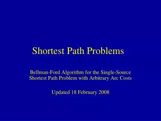
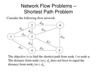
3. If H is a subgraph of a weighted graph, the weight w(H) of H is the sum of the weights on its edges. Many optimization problems amount to finding, in a weighted graph, a subgraph of a certain type with minimum (or maximum) weight. One such is the shortest path problem: given a railway network connecting various towns, determine a shortest route between two specified towns in the network.

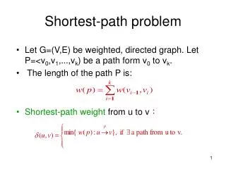
4. Here we must find, in a weighted graph, a path of minimum weight connecting two specified vertices u0 and v0 ; the weights represent distances by rail between directly- linked towns, and therefore non-negative. The path indicated in the next figure is a (u0 , v0) -path of minimum weight.

5. 1 2 b c d 9 9 7 5 3 2 6 8 1 8 2 a e f g h 4 1 7 2 1 4 1 i j k 9 1 Shortest Path: d(a,h)= 12

6. For clarity of exposition, we shall refer to the weight of a path in a weighted graphs as its length; similarly the minimum weight of a (u , v)-path will be called the distance between u and v and denoted by d(u , v). We shall assume here that G is simple, and all weights are positive. We adopt the convention that w(uv) =  if uv  E.

7. The algorithm to be described was discovered by Dijkstra (1959). It finds not only the shortest (u0 , v0)-path, but shortest paths from u0 to all other vertices in the graph (G).

8. Basic Idea The algorithm uses two sets of vertices, S and C. At every moment the set S contains those nodes that have already been chosen; as we shall see, the minimal distance from the source is already known for every node is S. The set C contains all the other nodes, whose minimal distance from the source is not known, and which are candidates to be chosen at some later stage. When the algorithm stops, S contains all the vertices of the graph and our problem is solved. At each step we choose the node in C whose distance to the source is least, and add it to S.

9. Dijkstra’s Shortest Path Algorithm l(v) - label of the vertex v 1. Set l(u0) = 0, l(v) =  for v  u0, S0 ={u0} and i = 0. 2. For each v not in Si, replace l(v) by min{l(v) , l(ui) + w(ui,v)}. Compute the minimum of the vertices not in Si and let ui+1 denote a vertex for which this minimum is attained. Set Si{ui+1}. 3. If i is one less than the number of vertices in a graph, stop. If i < v -1, replace i by i++ go to step 2.

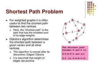
10. Example 4 We begin at vertex 0 and modify the labels of the adjacent vertices. 1 1 3 0 1 2 2 2 1 2 3 3

11. 4 1 1 3 0 1 2 2 2 1 2 3 3

12. 4 1 1 3 0 1 2 2 2 1 2 3 3

13. 4 1 1 3 0 1 2 2 2 1 2 3 3

14. 4 1 1 3 0 1 2 2 2 1 2 3 3 Shortest path from d(0,4) = 2 Path is: 0,1,4