Download
1 / 16
160 likes | 329 Vues
Lecture 7: QTL Mapping I: Inbred Line Crosses. P 1 x P 2. B 2. B 1. F 1. F 1. F 1 x F 1. F 1. F 1. Backcross design. Backcross design. F 2 design. F 2. F 2. Advanced intercross Design (AIC, AIC k ). F k. Experimental Design: Crosses. Experimental Designs: Marker Analysis.

E N D
Lecture 7:QTL Mapping I: Inbred Line Crosses
P1 x P2 B2 B1 F1 F1 F1 x F1 F1 F1 Backcross design Backcross design F2 design F2 F2 Advanced intercross Design (AIC, AICk) Fk Experimental Design: Crosses
Experimental Designs: Marker Analysis Single marker analysis Flanking marker analysis (interval mapping) Composite interval mapping Interval mapping plus additional markers Multipoint mapping Uses all markers on a chromosome simultaneously
P r ( Q M ) k j P r ( Q j M ) = k j P r ( M ) j Conditional Probabilities of QTL Genotypes The basic building block for all QTL methods is Pr(Qk | Mj) --- the probability of QTL genotype Qk given the marker genotype is Mj. Consider a QTL linked to a marker (recombination Fraction = c). Cross MMQQ x mmqq. In the F1, all gametes are MQ and mq In the F2, freq(MQ) = freq(mq) = (1-c)/2, freq(mQ) = freq(Mq) = c/2
Hence, Pr(MMQQ) = Pr(MQ)Pr(MQ) = (1-c)2/4 Pr(MMQq) = 2Pr(MQ)Pr(Mq) = 2c(1-c)/4 Pr(MMqq) = Pr(Mq)Pr(Mq) = c2 /4 Why the 2? MQ from father, Mq from mother, OR MQ from mother, Mq from father Since Pr(MM) = 1/4, the conditional probabilities become Pr(QQ | MM) = Pr(MMQQ)/Pr(MM) = (1-c)2 Pr(Qq | MM) = Pr(MMQq)/Pr(MM) = 2c(1-c) Pr(qq | MM) = Pr(MMqq)/Pr(MM) = c2
Q M2 M1 Genetic map c1 c2 c12 No interference: c12 = c1 + c2 - 2c1c2 Complete interference: c12 = c1 + c2 2 Marker loci Suppose the cross is M1M1QQM2M2 x m1m1qqm2m2 In F2, Pr(M1QM2) = (1-c1)(1-c2) Pr(M1Qm2) = (1-c1) c2 Pr(m1QM2) = (1-c1) c2 Likewise, Pr(M1M2) = 1-c12 = 1- c1 + c2 A little bookkeeping gives
2 2 ( 1 ° c ) ( 1 ° c ) 1 2 P r ( Q Q j M M M M ) = 1 1 2 2 ( 1 ° c ) 2 1 2 2 c c ( 1 ° c ) ( 1 ° c ) 1 2 1 2 P r ( Q q j M M M M ) = 1 1 2 2 2 ( 1 ° c ) 1 2 2 2 c c 1 2 P r ( q q j M M M M ) = 1 1 2 2 2 ( 1 ° c ) 1 2 - - - - - - -
N X π = π P r ( Q j M ) M Q k j j k k = 1 - - ( π ° π ) = 2 = a ( 1 ° 2 c ) M M m m Expected Marker Means The expected trait mean for marker genotype Mj is just For example, if QQ = 2a, Qa = a(1+k), qq = 0, then in the F2 of an MMQQ/mmqq cross, • If the trait mean is significantly different for the genotypes at a marker locus, it is linked to a QTL • A small MM-mm difference could be (i) a tightly-linked QTL of small effect or (ii) loose linkage to a large QTL
µ ∂ - - - π ° π 1 ° c ° c - M M M M m m m m 1 2 1 1 2 2 1 1 2 2 = a - - 2 1 ° c ° c + 2 c c 1 2 1 2 - ' a ( 1 ° 2 c c ) 1 2 ( µ ) ∂ - 1 π ° π - M M m m 1 1 1 1 This is essentially a for even modest linkage c = 1 ° 1 2 2 a ( µ ∂ ) - 1 π ° π - M M m m 1 1 1 1 ' 1 ° - 2 π ° π M M M M m m m m 1 1 2 2 1 1 2 2 Hence, the use of single markers provides for detection of a QTL. However, single marker means does not allow separate estimation of a and c. Now consider using interval mapping (flanking markers) Hence, a and c can be estimated from the mean values of flanking marker genotypes
z = π + b + e i k i i k Value of trait in kth individual of marker genotype type i Effect of marker genotype i on trait value Linear Models for QTL Detection The use of differences in the mean trait value for different marker genotypes to detect a QTL and estimate its effects is a use of linear models. One-way ANOVA. Detection: a QTL is linked to the marker if at least one of the bi is significantly different from zero Estimation (QTL effect and position): This requires relating the bi to the QTL effects and map position
z = π + a + b + d + e i k i k Effect from marker genotype at first marker set (can be > 1 loci) Effect from marker genotype at second marker set Interaction between marker genotypes i in 1st marker set and k in 2nd marker set Detecting epistasis One major advantage of linear models is their flexibility. To test for epistasis between two QTLs, used an ANOVA with an interaction term • At least one of the ai significantly different from 0 ---- QTL linked to first marker set • At least one of the bk significantly different from 0 ---- QTL linked to second marker set • At least one of the dik significantly different from 0 ---- interactions between QTL in sets 1 and two
N X 2 ` ( z j M ) = ' ( z ; π ; æ ) P r ( Q j M ) j Q k j k k = 1 Trait value given marker genotype is type j Distribution of trait value given QTL genotype is k is normal with mean mQk. (QTL effects enter here) Probability of QTL genotype k given marker genotype j --- genetic map and linkage phase entire here Sum over the N possible linked QTL genotypes Maximum Likelihood Methods ML methods use the entire distribution of the data, not just the marker genotype means. More powerful that linear models, but not as flexible in extending solutions (new analysis required for each model) Basic likelihood function: This is a mixture model
m a x ` ( z ) - r L R = ° 2 l n m a x ` ( z ) Maximum of the likelihood under a no-linked QTL model Maximum of the full likelihood } { ∑ ∏ m a x ` ( z ) L R ( c ) L R ( c ) - r L O D ( c ) = ° l o g = ' 1 0 m a x ` ( z ; c ) 2 l n 1 0 4 : 6 1 ML methods combine both detection and estimation Of QTL effects/position. Test for a linked QTL given from the LR test The LR score is often plotted by trying different locations for the QTL (I.e., values of c) and computing a LOD score for each
i-1 i i+1 i+2 CIM works by adding an additional term to the linear model , X b x k k j k 6 i ; i = + 1 Interval Mapping with Marker Cofactors Consider interval mapping using the markers i and i+1. QTLs linked to these markers, but outside this interval, can contribute (falsely) to estimation of QTL position and effect Now suppose we also add the two markers flanking the interval (i-1 and i+2) CIM also (potentially) includes unlinked markers to account for QTL on other chromosomes. Inclusion of markers i-1 and i+2 fully account for any linked QTLs to the left of i-1 and the right of i+2 Interval being mapped Interval mapping + marker cofactors is called Composite Interval Mapping (CIM) However, still do not account for QTLs in the areas
Power and Repeatability: The Beavis Effect QTLs with low power of detection tend to have their effects overestimated, often very dramatically As power of detection increases, the overestimation of detected QTLs becomes far less serious This is often called the Beavis Effect, after Bill Beavis who first noticed this in simulation studies