Optical tweezers and trap stiffness
220 likes | 479 Vues
Optical tweezers and trap stiffness. Dept. of Mechatronics Yong-Gu Lee. Bechhoefer J and Wilson S. 2002. Faster, cheaper, safer optical tweezers for the undergraduate laboratory. Am. J. Phys. 70: 393-400. Potential well of laser trapping. Escape force method.

Optical tweezers and trap stiffness
E N D
Presentation Transcript
Optical tweezers and trap stiffness Dept. of Mechatronics Yong-Gu Lee • Bechhoefer J and Wilson S. 2002. Faster, cheaper, safer optical tweezers for the undergraduate laboratory. Am. J. Phys. 70: 393-400.
Escape force method • This method determines the minimal force required to pull an object free of the trap entirely, generally accomplished by imposing a viscous drag force whose magnitude can be computed • To produce the necessary force, the particle may either be pulled through the fluid (by moving the trap relative to a stationary stage), or more conventionally, the fluid can be moved past the particle (by moving the stage relative to a stationary trap). • The particle velocity immediately after escape is measured from the video record, which permits an estimate of the escape force, provided that the viscous drag coefficient of the particle is known. While somewhat crude, this technique permits calibration of force to within about 10%. • Note that escape forces are determined by optical properties at the very edges of the trap, where the restoring force is no longer a linear function of the displacement. Since the measurement is not at the center of the trap, the trap stiffness cannot be ascertained. • Escape forces are generally somewhat different in the x,y,z directions, so the exact escape path must be determined for precise measurements. This calibration method does not require a position detector with nanometer resolution.
Drag Force Method • By applying a known viscous drag force, F, and measuring the displacement produced from the trap center, x, the stiffness k follows from k=F/x. • In practice, drag forces are usually produced by periodic movement of the microscope stage while holding the particle in a fixed trap: either triangle waves of displacement (corresponding to a square wave of force) or sine waves of displacement (corresponding to cosine waves of force) work well • Once trap stiffness is determined, optical forces can be computed from knowledge of the particle position relative to the trap center, provided that measurements are made within the linear (Hookeian) region of the trap. Apart from the need for a well-calibrated piezo stage and position detector, the viscous drag on the particle must be known.
Equipartition Method • One of the simplest and most straightforward ways of determining trap stiffness is to measure the thermal fluctuations in position of a trapped particle. The stiffness of the tweezers is then computed from the Equipartition theorem for a particle bound in a harmonic potential: • The chief advantage of this method is that knowledge of the viscous drag coefficient is not required (and therefore of the particle’s geometry as well as the fluid viscosity). A fast, wellcalibrated position detector is essential, precluding video-based schemes.
Step Response Method • The trap stiffness may also be determined by finding the response of a particle to a rapid, stepwise movement of the trap • For small steps of the trap, xt the response xb is given by below where is trap stiffness and is the viscous drag. • harder to identify extraneous sources of noise or artifact using this approach. The time constant for movement of the trap must be faster than the characteristic damping time of the particle
Trap stiffness calculation by power spectrum Ref. Bechhoefer J and Wilson S. 2002. Faster, cheaper, safer optical tweezers for the undergraduate laboratory. Am. J. Phys. 70: 393-400. Rolf Rysdyk, Automatic Control of Flight Vehicles class notes: stochastic signal models, http://www.aa.washington.edu/research/afsl/coursework/aa518/aa518.shtml
Normal probability distribution • If the values of x are normally distributed about a zero mean, then ‘histogram’ distribution x would look like: where is the variance and N is the number of samplings that is sufficiently large.
A particle immersed in a fluid and trapped in a harmonic potential undergoes following dynamics
If the particle is a sphere of radius R immersed in a fluid of viscosity and far from any boundaries, then standard hydrodynamic arguments lead to • For scanning optical tweezers the velocity of the scan must satisfy [dimension, kg/s] Viscosity [dimension, Stress* Time, ]
Assume overdamped motion :general solution Ref. Paul D. Ritger and Nicholas J. Rose, Differential equations with applications, McGraw-Hill, 1968, pp. 40-41
Autocorrelation • The correlation of a signal y(t) with itself is referred to as autocorrelation. Consider there is a time delay during the correlation,
Autocorrelation function • Autocorrelation function Note we have replaced t by 0, this is allowed because we are assuming that we are assuming that x(t) is a stationary stochastic process, so that ensemble averages are independent of the time at which they are carried out
Autocorrelation function is then obtained by taking an ensemble average, bearing in mind that the only stochastic (random) term is
Since successive random kicks are uncorrelated with each other
The final form of the autocorrelation function and power spectral density Using Wiender-Khintchine theorem, one can calculate the power spectrum of the particle by taking the Fourier transform of above to find Corner frequency which gives the characteristic frequency response of the particle to the thermal driving force, normalized so that
Wiener-Khinchin Theorem Ref. Weisstein, Eric W. "Wiener-Khinchin Theorem." From MathWorld— A Wolfram Web Resource. http://mathworld.wolfram.com/Wiener-KhinchinTheorem.html
Measurement from experiments Arbitrary units is sufficient Power spectrum obtained for a 1 micrometer big polystyrene bead in a trap. Taken from http://www.nbi.dk/~tweezer/introduction.htm