Forecasting using trend analysis
Forecasting using trend analysis. Part 1. Theory Part 2. Using Excel: a demonstration. Assignment 1, 2. Learning objectives. To compute a trend for a given time-series data using Excel To choose a best fitting trend line for a given time-series

Forecasting using trend analysis
E N D
Presentation Transcript
Forecasting using trend analysis • Part 1. Theory • Part 2. Using Excel: a demonstration. • Assignment 1, 2
Learning objectives • To compute a trend for a given time-series data using Excel • To choose a best fitting trend line for a given time-series • To calculate a forecast using regression equation To learn how:
Main idea of the trend analysis forecasting method • Main idea of the method: a forecast is calculated by inserting a time value into the regression equation. The regression equation is determined from the time-serieas data using the “least squares method”
Prerequisites: 2. Correlation There should be a sufficient correlation between the time parameter and the values of the time-series data
The Correlation Coefficient • The correlation coefficient, R, measure the strength and direction of linear relationships between two variables. It has a value between –1 and +1 • A correlation near zero indicates little linear relationship, and a correlation near one indicates a strong linear relationship between the two variables
Main idea of the trend analysis method • Trend analysis uses a technique called least squares to fit a trend line to a set of time series data and then project the line into the future for a forecast. • Trend analysis is a special case of regression analysis where the dependent variable is the variable to be forecasted and the independent variable is time. • While moving average model limits the forecast to one period in the future, trend analysis is a technique for making forecasts further than one period into the future.
The general equation for a trend line F=a+bt Where: • F – forecast, • t – time value, • a – y intercept, • b – slope of the line.
Least Square Method • Least square method determines the values for a and b so that the resulting line is the best-fit line through a set of the historical data. • After a and b have been determined, the equation can be used to forecast future values.
Statistical measures of goodness of fit • The Correlation Coefficient • The Determination Coefficient In trend analysis the following measures will be used:
The Coefficient of Determination • The coefficient of determination, R2, measures the percentage of variaion in the dependent variable that is explained by the regression or trend line. It has a value between zero and one, with a high value indicating a good fit.
Goodness of fitt: Determination Coefficient RSQ • Range: [0, 1]. • RSQ=1 means best fitting; • RSQ=0 means worse fitting;
Evaluation of the trend analysis forecasting method • Advantages: Simple to use (if using appropriate software) • Disadvantages: 1) not always applicable for the long-term time series (because there exist several ternds in such cases); 2) not applicable for seasonal and cyclic datta patterns.
Part 2. Switch to Excel Open a Workbook trend.xls, save it to your computer
Working with Excel • Demonstration of the forecasting procedure using trend analysis method • Assignment 1. Repeating of the forecasting procedure with the same data • Assignment 2. Forecasting of the expenditure
Using Excel to calculate linear trend • Select a line on the diagram • Right click and select Add Trendline • Select a type of the trend (Linear)
Non-linear trends • Logarythmic • Polynomial • Power • Exponential Excel provides easy calculation of the following trends
Choosing the trend that fitts best • 1) Roughly: Visually, comparing the data pattern to the one of the 5 trends (linear, logarythmic, polynomial, power, exponential) • 2) In a detailed way: By means of the determination coefficient

