Graphs
Graphs. Graphs are not function plots. Example:. a. b. V = {a,b,c,d,e} E = {(a,b),(a,c),(a,d), (b,e),(c,d),(c,e), (d,e)}. c. e. d. What is a Graph?. A graph G is a pair ( V , E ) where V : set of vertices E : set of edges connecting the vertices in V

Graphs
E N D
Presentation Transcript
Example: a b V= {a,b,c,d,e} E= {(a,b),(a,c),(a,d), (b,e),(c,d),(c,e), (d,e)} c e d What is a Graph? • A graph G is a pair (V,E) where V: set of vertices E: set of edges connecting the vertices in V Vertices and edges are positions and store elements • An edge e = (u,v) is a pair of vertices • Graph is a more general data structure. Tree is a special case of graph
A vertex represents an airport and stores the three-letter airport code An edge represents a flight route between two airports and stores the mileage of the route Graph: Example 849 PVD 1843 ORD 142 SFO 802 LGA 1743 337 1387 HNL 2555 950 1233 LAX 1120 DFW MCO
Graph: Examples Graphics Vision math.ucf.edu • Computer networks • Local area network • Internet • Web • Electronic circuits • Printed circuit board • Integrated circuit • Transportation networks • Highway network • Flight network • Databases • Entity-relationship diagram cs.ucf.edu ucf.edu sprint.net att.net ATI.com John Paul David
Edge Types • Directed edge • ordered pair of vertices (u,v) • first vertex u is the origin • second vertex v is the destination • e.g., a flight • Undirected edge • unordered pair of vertices (u,v) • e.g., a flight route • Directed graph • all the edges are directed • e.g., flight network • Undirected graph • all the edges are undirected • e.g., route network flight AA 1348 MCO LGA 950 miles MCO LGA
a a b b c c e d e d a b e d c b e d c Graph Terminology 3 2 a b • adjacent vertices: vertices connected by an edge • degree (of a vertex): # of adjacent vertices NOTE: The sum of the degrees of all vertices is twice the number of edges. Why? Since adjacent vertices each count the adjoining edge, it will be counted twice • path: sequence of vertices v1,v2,. . .vk such that consecutive vertices vi and vi+1 are adjacent. 3 c 3 3 d e
a b b e c c e d a c d a More Graph Terminology • simple path: no repeated vertices • cycle: simple path, except that the last vertex is the same as the first vertex
Subgraphs • A subgraph S of a graph G is a graph such that • The vertices of S are a subset of the vertices of G • The edges of S are a subset of the edges of G • A spanning subgraph of G is a subgraph that contains all the vertices of G Subgraph Spanning subgraph
A graph is connected if there is a path between every pair of vertices A connected component of a graph G is a connected subgraph of G Connectivity Connected graph Non connected graph with two connected components
A graph is complete if all pair of vertices are adjacent Connectivity Complete graph Let n = #vertices, and m= #edges How many total edges in a complete graph? Each of the n vertices is incident to n-1 edges, however, we would have counted each edge twice!!! Therefore, intuitively, m = n(n -1)/2. Therefore, if a graph is not complete, m < n(n -1)/2
Tree Forest Trees and Forests • A forest is an undirected graph without cycles • The connected components of a forest are trees • A (free) tree is an undirected graph T such that • T is connected • T has no cycles This definition of tree is different from the one of a rooted tree
Tree Forest Trees and Forests Let n = #vertices, and m= #edges How many total edges in a tree? m = n - 1 Total edges in a forest? m < n - 1
Spanning Trees and Forests • A spanning tree of a connected graph is a spanning subgraph that is a tree • A spanning tree is not unique unless the graph is a tree • A spanning forest of a graph is a spanning subgraph that is a forest Graph Spanning tree
Data Structures for Graphs • A Graph! How can we represent it? • Edge list • Adjacency lists • Adjacency matrix
NW 35 DL 247 AA 49 DL 335 AA 1387 AA 523 AA 41 1 UA 120 AA 903 UA 877 TW 45 E V BOS LAX DFW JFK MIA ORD SFO Edge List • The edge list structure simply stores the vertices and the edges into two containers (ex: lists, vectors etc..) • each edge object has references to the vertices it connects. Easy to implement. Space = O(n+m) Finding the edges incident on a given vertex is inefficient since it requires examining the entire edge sequence. Time: O(m)
a b c e d a c b d b a e c a e d d a c e e c b d Adjacency List (traditional) • adjacency list of a vertex v: sequence of vertices adjacent to v • represent the graph by the adjacency lists of all the vertices Space = (n + deg(v)) = (n + m)
NW 35 DL 247 AA 49 DL 335 AA 1387 AA 523 AA 41 1 UA 120 AA 903 UA 877 TW 45 E V BOS LAX DFW JFK MIA ORD SFO Adjacency List (modern) • The adjacency list structure extends the edge list structure by adding incidence containers to each vertex. space is O(n + m). in out in out in out in out in out in out in out NW 35 AA 49 UA 120 AA1387 DL335 NW 35 AA1387 DL 247 AA523 UA 120 UA 877 TW 45 DL 247 AA 41 1 UA 877 AA 49 AA 903 AA 903 AA 41 1 DL 335 AA 523 TW 45
a b c d e a b a F T T T F b T F F F T c T F F T T c d T F T F T e F T T T F d e d Adjacency Matrix (traditional) • matrix M with entries for all pairs of vertices • M[i,j] = true means that there is an edge (i,j) in the graph. • M[i,j] = false means that there is no edge (i,j) in the graph. • There is an entry for every possible edge, therefore: Space = (n2)
Adjacency Matrix (modern) • The adjacency matrix structures augments the edge list structure with a matrix where each row and column corresponds to a vertex.
Data Structures for Graphs • A Graph! How can we represent it? • Edge list • Adjacency lists • Adjacency matrix
NW 35 DL 247 AA 49 DL 335 AA 1387 AA 523 AA 41 1 UA 120 AA 903 UA 877 TW 45 E V BOS LAX DFW JFK MIA ORD SFO Edge List • The edge list structure simply stores the vertices and the edges into two containers (ex: lists, vectors etc..) • each edge object has references to the vertices it connects. Easy to implement. Space = O(n+m) Finding the edges incident on a given vertex is inefficient since it requires examining the entire edge sequence. Time: O(m)
NW 35 DL 247 AA 49 DL 335 AA 1387 AA 523 AA 41 1 UA 120 AA 903 UA 877 TW 45 E V BOS LAX DFW JFK MIA ORD SFO Adjacency List • The adjacency list structure extends the edge list structure by adding incidence containers to each vertex. space is O(n + m). in out in out in out in out in out in out in out NW 35 AA 49 UA 120 AA1387 DL335 NW 35 AA1387 DL 247 AA523 UA 120 UA 877 TW 45 DL 247 AA 41 1 UA 877 AA 49 AA 903 AA 903 AA 41 1 DL 335 AA 523 TW 45
Adjacency Matrix • The adjacency matrix structures augments the edge list structure with a matrix where each row and column corresponds to a vertex.
Graph Traversal • A procedure for exploring a graph by examining all of its vertices and edges. • Two different techniques: • Depth First traversal (DFT) • Breadth First Traversal (BFT)
Depth-First Search • Depth-first search (DFS) is a general technique for traversing a graph • A DFS traversal of a graph G • Visits all the vertices and edges of G • Determines whether G is connected • Computes the connected components of G • Computes a spanning forest of G
A B D E C A A A B D E B D E B D E C C C Example unexplored vertex A visited vertex A unexplored edge discovery edge back edge
A A A B D E B D E B D E C C C A B D E C Example (cont.)
DFS Algorithm • The algorithm uses a mechanism for setting and getting “labels” of vertices and edges AlgorithmDFS(G, v) Input graph Gand a start vertexv of G Output labeling of the edges of G in the connected component of v as discovery edges and back edges setLabel(v, VISITED) for alle G.incidentEdges(v) ifgetLabel(e) = UNEXPLORED w opposite(v,e) if getLabel(w) = UNEXPLORED setLabel(e, DISCOVERY) DFS(G, w) else setLabel(e, BACK) AlgorithmDFS(G) Input graph G Output labeling of the edges of G as discovery edges and back edges for allu G.vertices() setLabel(u, UNEXPLORED) for alle G.edges() setLabel(e, UNEXPLORED) for allv G.vertices() ifgetLabel(v) = UNEXPLORED DFS(G, v)
Property 1 DFS(G, v) visits all the vertices and edges in the connected component of v Property 2 The discovery edges labeled by DFS(G, v) form a spanning tree of the connected component of v A B D E C Properties of DFS
Setting/getting a vertex/edge label takes O(1) time Each vertex is labeled twice once as UNEXPLORED once as VISITED Each edge is labeled twice once as UNEXPLORED once as DISCOVERY or BACK DFS runs in O(n+m) time provided the graph is represented by the adjacency list structure Analysis of DFS
DFS on a graph with n vertices and m edges takes O(n + m ) time DFS can be further extended to solve other graph problems Find and report a path between two given vertices Find a cycle in the graph Depth-First Search
Path Finding • We call DFS(G, u) with u as the start vertex • We use a stack S to keep track of the path between the start vertex and the current vertex • As soon as destination vertex v is encountered, we return the path as the contents of the stack
Path Finding AlgorithmpathDFS(G, v, z) setLabel(v, VISITED) S.push(v) if v= z return S.elements() for all e G.incidentEdges(v) ifgetLabel(e) = UNEXPLORED w opposite(v,e) if getLabel(w) = UNEXPLORED setLabel(e, DISCOVERY) S.push(e) pathDFS(G, w, z) S.pop(e) else setLabel(e, BACK) S.pop(v)
Cycle Finding • We use a stack S to keep track of the path between the start vertex and the current vertex • As soon as a back edge (v, w) is encountered, we return the cycle as the portion of the stack from the top to vertex w
Cycle Finding AlgorithmcycleDFS(G, v, z) setLabel(v, VISITED) S.push(v) for all e G.incidentEdges(v) ifgetLabel(e) = UNEXPLORED w opposite(v,e) S.push(e) if getLabel(w) = UNEXPLORED setLabel(e, DISCOVERY) pathDFS(G, w, z) S.pop(e) else T new empty stack repeat o S.pop() T.push(o) until o= w return T.elements() S.pop(v)
a-b pa | pb a-c pa | pc a-d pa | pd b-e pb | pe c-d pc | pd c-e pc | pe d-e pd | pe a b a c e b d c pa-b pa-c pa-d pa-b pb-e pa-c pc-d pc-e pa-d pc-d pd-e pb-e pc-e pd-e e d Review: Representation Space = (n + deg(v)) = (n + m)
a-b pa | pb a-c pa | pc a-d pa | pd b-e pb | pe c-d pc | pd c-e pc | pe d-e pd | pe a c e b d pa-b pa-c pa-d pa-b pb-e pa-c pc-d pc-e pa-d pc-d pd-e pb-e pc-e pd-e Review: DFS a b c e d
a-b pa | pb a-c pa | pc a-d pa | pd b-e pb | pe c-d pc | pd c-e pc | pe d-e pd | pe a c e b d pa-b pa-c pa-d pa-b pb-e pa-c pc-d pc-e pa-d pc-d pd-e pb-e pc-e pd-e Review: DFS a b c e d
a-b pa | pb a-c pa | pc a-d pa | pd b-e pb | pe c-d pc | pd c-e pc | pe d-e pd | pe a c e b d pa-b pa-c pa-d pa-b pb-e pa-c pc-d pc-e pa-d pc-d pd-e pb-e pc-e pd-e Review: DFS a b c e d
a-b pa | pb a-c pa | pc a-d pa | pd b-e pb | pe c-d pc | pd c-e pc | pe d-e pd | pe a c e b d pa-b pa-c pa-d pa-b pb-e pa-c pc-d pc-e pa-d pc-d pd-e pb-e pc-e pd-e Review: DFS a b c e d
a-b pa | pb a-c pa | pc a-d pa | pd b-e pb | pe c-d pc | pd c-e pc | pe d-e pd | pe a c e b d pa-b pa-c pa-d pa-b pb-e pa-c pc-d pc-e pa-d pc-d pd-e pb-e pc-e pd-e Review: DFS a b c e d
a-b pa | pb a-c pa | pc a-d pa | pd b-e pb | pe c-d pc | pd c-e pc | pe d-e pd | pe a c e b d pa-b pa-c pa-d pa-b pb-e pa-c pc-d pc-e pa-d pc-d pd-e pb-e pc-e pd-e Review: DFS a b c e d
a-b pa | pb a-c pa | pc a-d pa | pd b-e pb | pe c-d pc | pd c-e pc | pe d-e pd | pe a c e b d pa-b pa-c pa-d pa-b pb-e pa-c pc-d pc-e pa-d pc-d pd-e pb-e pc-e pd-e Review: DFS a b c e d
a-b pa | pb a-c pa | pc a-d pa | pd b-e pb | pe c-d pc | pd c-e pc | pe d-e pd | pe a c e b d pa-b pa-c pa-d pa-b pb-e pa-c pc-d pc-e pa-d pc-d pd-e pb-e pc-e pd-e Review: DFS a b c e d
a-b pa | pb a-c pa | pc a-d pa | pd b-e pb | pe c-d pc | pd c-e pc | pe d-e pd | pe a c e b d pa-b pa-c pa-d pa-b pb-e pa-c pc-d pc-e pa-d pc-d pd-e pb-e pc-e pd-e Review: DFS a b c e d
a-b pa | pb a-c pa | pc a-d pa | pd b-e pb | pe c-d pc | pd c-e pc | pe d-e pd | pe a c e b d pa-b pa-c pa-d pa-b pb-e pa-c pc-d pc-e pa-d pc-d pd-e pb-e pc-e pd-e Review: DFS a b c e d
a-b pa | pb a-c pa | pc a-d pa | pd b-e pb | pe c-d pc | pd c-e pc | pe d-e pd | pe a c e b d pa-b pa-c pa-d pa-b pb-e pa-c pc-d pc-e pa-d pc-d pd-e pb-e pc-e pd-e Review: DFS a b c e d
a-b pa | pb a-c pa | pc a-d pa | pd b-e pb | pe c-d pc | pd c-e pc | pe d-e pd | pe a c e b d pa-b pa-c pa-d pa-b pb-e pa-c pc-d pc-e pa-d pc-d pd-e pb-e pc-e pd-e Review: DFS a b c e d
a-b pa | pb a-c pa | pc a-d pa | pd b-e pb | pe c-d pc | pd c-e pc | pe d-e pd | pe a c e b d pa-b pa-c pa-d pa-b pb-e pa-c pc-d pc-e pa-d pc-d pd-e pb-e pc-e pd-e Review: DFS a b c e d