Download

1 / 31
320 likes | 469 Vues
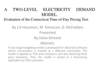
A Two-Level Electricity Demand Model. Hausman , Kinnucan , and Mcfadden. Introduction. Analyzed the Connecticut Peak Load Pricing Test Oct 1975 to Oct 1976 199 Households Meters installed to measure electricity consumption Faced a peak load pricing system with 3 prices

E N D
A Two-Level Electricity Demand Model Hausman, Kinnucan, and Mcfadden
Introduction • Analyzed the Connecticut Peak Load Pricing Test • Oct 1975 to Oct 1976 • 199 Households • Meters installed to measure electricity consumption • Faced a peak load pricing system with 3 prices • 16 cents / kwh peak, 3 cents / kwh intermediate, 1 cent / kwh off-peak.
Procedure • Determine household preference for amount to spend on electricity • Estimate the cost of that electricity based on time of consumption (TOD pricing) or previous rate structure (controls) • Determine from relative demand and pricing, the total demand
Technique • Estimate consumer demand w/ two stage budget • Treat electricity demand within each period as a separate commodity • Estimate demand across periods conditioned on relative prices, appliance stock, household characteristics, and environmental effects
Technique • Estimate a price index for electricity • Household consumption determined by price of electricity and prices for other goods • Absolute demand is derived from relative demand and price index
Two Level Budgeting Model imposes seperability between consumption of electricity and other commodities • Decides how much to spend on electricity and all other goods
Derivation of Time of Day Model • Distribution of relative load across households more stable than consumption levels • Two level budgeting model • Reduces complication of controls (due to declining block tariff) • Requires linear homogeneity • Considers household electricity consumption in a representative day. • Appliance mix is assumed exogenous, therefore no effect on consumption patterns • Seasonality ignored • Interday effects ignored • Rates do not change with consumption only time of day.
Derivation of time of day model • Assume: • Utility determined by vector of electricity consumption at different times of day, and consumption of all other goods (x0) • HH decides how much to spend on electricity and how much to spend on other commodities • Total consumption then depends on price of electricity
Derivation of Time of Day Model • Divide day into series of 15 minute periods • Vector of electricity rates with a price corresponding to each period • Indirect utility function: • Utility function from with assumptions: • Utility function for electricity • Where , total electricity expendature
Derivation • Indirect utility function • Use Roy’s identity, linear homogeneity and Eulers theorem to get demand function
Derivation • Proportion of total consumption in base period • Consumption in any period relative to base period is
Derivation • Taylor expansion gives • Full accounting gives single period cons. func
Derivation • Price index to use in consumption function determined by total electricity consumption and total consumption.
Derivation • Used to derive demand function for total daily demand: • Pre-experimental period, price constant on all periods, but is a function of monthly demand due to declining block rate structure.
Estimation • Sample of 150 households used • 20 not used to estimate, but used to test • Two levels of demand estimated • Estimated with daily data using demand equation • Estimated price index (post exp) or insturmental variables (pre exp) used to estimate consumption equation
Problems • Not a random sample • Chosen based on an endogenous variable • Residuals surely correlated with RHS vars • Inverse sample weights (WLS) used to correct for this issue • Estimates not efficient • Downward biased standard errors • Voluntary participation • Unobserved attributes determine participation, cannot be checked • Aigner and Hausman(1978) find that elasticity lower when not subject to voluntary choice, thus here, elasticity may be overstated.
Estimation • First level • Hourly demand equations • Estimated from 4 periods, weekdays and weekends during 2 winter months and 2 summer months, corresponding to system peak demand periods. • 11pm – 7am is base period
Results • Reported results for 3 representative periods, peak, off peak and intermediate • Coefficients from demand equation are all relative to base periods • Not accounting for long run substitution
Findings • Appliance coefficients have correct sign • Range / clothes dryer should be positive, since they will be operated during the day • Range use lower when facing peak pricing, moved to intermediate period • Freezer should have negative coefficient since it operates all the time, this increases the base period demand for the household. • Heater has spillover effects • Households used less heat energy during peak periods, lower demand spills over to non peak periods because people don’t readjust the thermostat
Findings • Elasticities are negative • 9-11 am more elastic than 5-7 pm • Intermediate period elasticities are lowest near peak periods • Day of the week variables suggest demand changes occur more during the day and less between days • First state equation is reasonable
Price index estimate • Compared pre experimental rates to post experimental price index • Treat declining block rate structure as linear two part tariff • Lump sum $6.46, marginal price is 3.54 cents / kwh • Experimental period prices come from price index equation, using estimated coefficients from demand equation estimate • Winter weekdays: 3.89 cents / kwh • High: 4.66 cents/kwh; Low: 3.25 cents/kwh
Price Index Estimate • Comparing experimental period to pre experimental period: • Households faced higher marginal cost by ~16% but no lump sum payment during experiment • Decrease in consumption did occur • 1% from previous year and 5% decline from controls • Increase in marginal prices outweighs the removal of lump sum payment
Estimation • Second Level • Daily demand equations • 4 demand estimates • Weekday / weekend, winter / summer • Less precise than first level estimates • Coefficients generally have correct total effect • Presence of electric heat adds consumption during winter • 1% rise in MP leads to reduction of weekday consumption by ~4.3% • Freezer adds to consumption, but elasticity is not significant, indicating non-discretionary nature of this appliance
Validation • Used 20 households from original sample to test predictive capacity of model • Forecasts do well in peak pricing periods forecasting relative load, though not significant • Large forecast errors for other periods, insignificant results, less important
Validation • When aggregated by period, forecasts appear accurate • Peak usage in validation group occurs in non-peak pricing period. Model correctly predicts this
Validation • Next, use forecasted price indices to forecast demand • Over prediction for low demand customers • Under prediction for high demand customers • Even when authors correct for sample issues, results are not significant • Second level (daily demand) not as reliable as first level (hourly demand) equations
Validation • Load forecasts better in peak than non peak periods • Smaller errors in peak periods forecast load reasonably well