Download
1 / 22
220 likes | 584 Vues
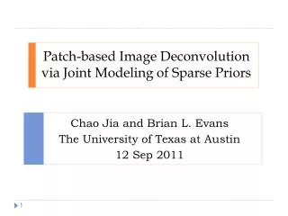
Patch-based Image Deconvolution via Joint Modeling of Sparse Priors . Chao Jia and Brian L. Evans The University of Texas at Austin 12 Sep 2011. Non-blind Image Deconvolution. Reconstruct natural image from blurred version Camera shake; astronomy; biomedical image reconstruction

E N D
Patch-based Image Deconvolution via Joint Modeling of Sparse Priors Chao Jia and Brian L. Evans The University of Texas at Austin 12 Sep 2011
Non-blind Image Deconvolution • Reconstruct natural image from blurred version • Camera shake; astronomy; biomedical image reconstruction • 2D convolution matrix H and Gaussian additive noise vector n • Maximum a-posteriori (MAP) estimation for vector X • Prior model for p(X) for natural images? [Elad 2007] • Optimization method?
Analysis-based modeling [Krishnan 2009] • Prior based on hyper-Laplacian distribution of the spatial derivative of natural images • Linear filtering to compute spatial derivative • Fit (0.5-0.8) and (normalization factor) to empirical data
Patch-based modeling • Sparse coding of patches • Spatial receptive fields of visual cortex [Olshausen 1997] • For 10 10 patches • Learn an overcomplete dictionary from natural images. • Application in image restoration • Denoising, superresolution[Yang 2010] • Localized algorithm: patches canoverlap • Use this model in deconvolution? [Lee 2007]
Prior model in natural images • From local to global • Slow convergence (EM Algorithm) • Patches should not overlap (Why?) boundary artifacts
Accelerate convergence Keep consistency on the boundary of adjacent patches Joint modeling Patch-based sparse coding Sparse spatial gradient • Take advantage of patch-based sparse representation while resolving the problems in? • Combine analysis-based prior and synthesis-based prior Keep details and textures
Joint modeling • Discard the generative model • Prior probability • After training, we fix the parameters for all images sparsity of gradients compatibility term sparsity of representation coefficients
MAP estimation using the joint model • Problem: • Iteratively updating w and X until convergence • w sub-problem small-scale L1 regularized square loss minimization • X sub-problem Half-quadratic splitting [Krishnan 2009] likelihood prior
Experimental results • Initialization: Wiener estimates / blurred images • Dictionary: learned from Berkeley Segmentation database • Patch size 12 12 • Prior parameters: • Runtime: (Matlab) 16s with Intel Core2 Duo CPU @2.26GHz • Experiment settings:
Experimental results PASCAL Visual Object Classes Challenge (VOC) 2007 database
Experimental results [Krishnan 2009] Original image [Portilla 2009] keeps more brick textures Blurred image Proposed
Experimental results • Textures zoomed in Original image [Krishnan 2009] [Portilla 2009] Proposed
Conclusions • Global model for MAP estimation • Able to solve general non-blind image deconvolution • Joint model of image pixels and representation coefficients • Sparsity of spatial derivative (analysis-based) • Sparsity of representation of patches in overcomplete dictionary (synthesis-based) • Iterative algorithm • converges in a few iterations • Matlab code for the proposed method is available at http://users.ece.utexas.edu/~bevans/papers/2011/sparsity/
References • [Elad 2007] M. Elad, P. Milanfar and R. Rubinstein, “Analysis versus synthesis in signal priors”, Inverse Problems, vol. 23, 2007. • [Krishnan 2009] D. Krishnan and R. Fergus, “Fast image deconvolution using hyper-Laplacian priors,” Advances in Neural Information Processing Systems, vol. 22, pp. 1-9, 2009. • [Olshausen 1997] B.A. Olshausen and D.J. Field, “Sparse coding with an overcomplete basis set: a strategy employed by V1,” Vision Research, vol. 37, no. 23, pp. 3311-3325, 1997. • [Portilla 2009] J. Portilla, “Image restoration through L0 analysis-based sparse optimization in tight frames,” in Proc. IEEE Int. Conf. on Image Processing, 2009, pp. 3909-3912. • [Yang 2010] J. yang, J. Wright, T.S. Huang and Y. Ma, “Image super-resolution via sparse representation,” IEEE Trans. on Image Processing, vol. 19, no. 11, pp. 2861-2873, 2010.
w sub-problem patches do not overlap small-scale l1 regularized square loss minimization
X sub-problem • Conjugate gradientiteratively reweighted least squares • Half-quadratic splitting [Krishnan 2009] auxiliary variable No need to solve the equation component-wise quartic function
blurred image; noise level; blurring kernel; initialization of recovered image MAP estimation using the joint model Update the coefficient of patches (w sub-problem) finish X sub-problem α>αmax ? Set α=α0 X converges? Update auxiliary variable Y (quartic equation) Update image X (FFT) α=kα
Image Quality Assessment • Full reference metric • ISNR -- increment in PSNR (peak signal-to-noise ratio) • SSIM -- structural similarity [Wang 2004]
Prior model of natural images • Analysis-based prior • Fast convergence • Over smooth the images • Synthesis-based prior (patch-based sparse representation) • Dictionary well adapted to nature images • Captures textures well • Slow convergence • Boundary artifacts
Computational complexity • Computational complexity • For each iteration: • N is the total number of pixels in the image • Average runtime comparison