
Image Stitching for Computational Photography
E N D
Presentation Transcript
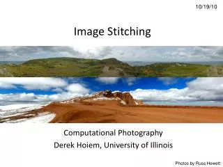
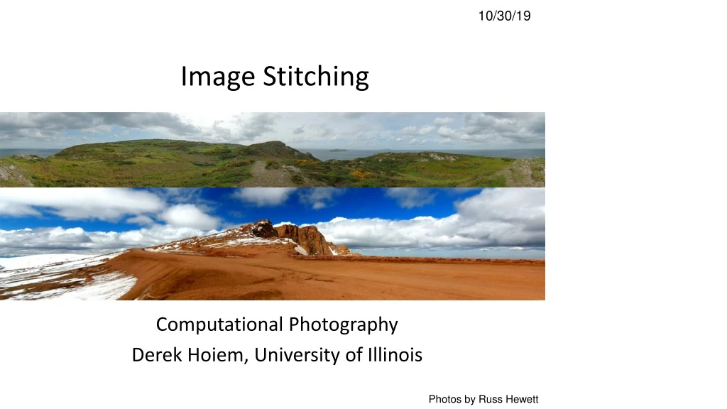
10/30/19 Image Stitching Computational Photography Derek Hoiem, University of Illinois Photos by Russ Hewett
My good excuse for not teaching Friday…(thank you Wilfredo!) Rowan Maeve
Project 3 Highlights • https://ksharma.web.illinois.edu/cs445/proj3/ (most likes) good octopus, laplacian image result • https://xz2.web.illinois.edu/cs445/proj3/ great main result • https://ayuship2.web.illinois.edu/cs445/proj3/ many great blends • https://liwenwu2.web.illinois.edu/cs445/proj3/ good blends, colorization • https://aipark2.web.illinois.edu/cs445/proj3/ good comparisons w/ web page design • https://byhsieh2.web.illinois.edu/cs445/proj3/ great blends and npr • https://yicheng9.web.illinois.edu/cs445/proj3/ cat bread and cat magic • https://kl2.web.illinois.edu/cs445/proj3/ mixed gradient • http://lehan2.web.illinois.edu/cs445/proj3/laplacian pyramid(the last one) • https://rxian2.web.illinois.edu/cs445/proj3/ duck and fish • https://yilinma3.web.illinois.edu/cs445/proj3/ the skate boy on the moon • https://wyang52.web.illinois.edu/cs445/proj3/rose • https://xiaoyis2.web.illinois.edu/cs445/proj3/ ship in the desert • https://sarwade2.web.illinois.edu/cs445/proj3/ Eiffel Candle
Laplacian pyramid Kartikeya Sharma
Anbang Ye Ayushi Patel Xiaohua Zhang Liwen Wu
Image Stitching Computational Photography Derek Hoiem, University of Illinois Photos by Russ Hewett
Project 5 Input video: https://www.youtube.com/watch?v=agI5za_gHHU Aligned frames: https://www.youtube.com/watch?v=Uahy6kPotaE Background: https://www.youtube.com/watch?v=Vt9vv1zCnLA Foreground: https://www.youtube.com/watch?v=OICkKNndEt4
Last Class: Keypoint Matching 1. Find a set of distinctive key- points 2. Define a region around each keypoint A1 B3 3. Extract and normalize the region content A2 A3 B2 B1 4. Compute a local descriptor from the normalized region 5. Match local descriptors K. Grauman, B. Leibe
Last Class: Summary • Keypoint detection: repeatable and distinctive • Corners, blobs • Harris, DoG • Descriptors: robust and selective • SIFT: spatial histograms of gradient orientation
Today: Image Stitching • Combine two or more overlapping images to make one larger image Add example Slide credit: Vaibhav Vaish
Views from rotating camera Camera Center
Correspondence of rotating camera . X • x = K [R t] X • x’ = K’ [R’ t’] X • t=t’=0 • x’=Hxwhere H = K’ R’ R-1 K-1 • Typically only R and f will change (4 parameters), but, in general, H has 8 parameters x x' f f'
Image Stitching Algorithm Overview • Detect keypoints • Match keypoints • Estimate homography with four matched keypoints (using RANSAC) • Project onto a surface and blend
Image Stitching Algorithm Overview • Detect/extract keypoints (e.g., DoG/SIFT) • Match keypoints (most similar features, compared to 2nd most similar)
Computing homography Assume we have four matched points: How do we compute homographyH? Direct Linear Transformation (DLT)
Computing homography Direct Linear Transform • Apply SVD: UDVT= A • h = Vsmallest (column of V corr. to smallest singular value) Matlab [U, S, V] = svd(A); h = V(:, end);
Computing homography Assume we have four matched points: How do we compute homographyH? Normalized DLT • Normalize coordinates for each image • Translate for zero mean • Scale so that u and v are ~=1 on average • This makes problem better behaved numerically (see Hartley and Zisserman p. 107-108) • Compute using DLT in normalized coordinates • Unnormalize:
Computing homography • Assume we have matched points with outliers: How do we compute homographyH? Automatic Homography Estimation with RANSAC
RANSAC: RANdomSAmple Consensus Scenario: We’ve got way more matched points than needed to fit the parameters, but we’re not sure which are correct RANSAC Algorithm • Repeat N times • Randomly select a sample • Select just enough points to recover the parameters • Fit the model with random sample • See how many other points agree • Best estimate is one with most agreement • can use agreeing points to refine estimate
Computing homography • Assume we have matched points with outliers: How do we compute homographyH? Automatic Homography Estimation with RANSAC • Choose number of iterations N • Choose 4 random potential matches • Compute H using normalized DLT • Project points from x to x’ for each potentially matching pair: • Count points with projected distance < t • E.g., t = 3 pixels • Repeat steps 2-5 N times • Choose H with most inliers HZ Tutorial ‘99
Automatic Image Stitching • Compute interest points on each image • Find candidate matches • Estimate homographyH using matched points and RANSAC with normalized DLT • Project each image onto the same surface and blend
Choosing a Projection Surface Many to choose: planar, cylindrical, spherical, cubic, etc.
Planar Mapping x x f f For red image: pixels are already on the planar surface For green image: map to first image plane
Planar Projection Planar Photos by Russ Hewett
Planar Projection Planar
Cylindrical Mapping x x f f For red image: compute h, theta on cylindrical surface from (u, v) For green image: map to first image plane, than map to cylindrical surface
Cylindrical Projection Cylindrical
Cylindrical Projection Cylindrical
Planar vs. Cylindrical Projection Planar Cylindrical
Recognizing Panoramas Brown and Lowe 2003, 2007 Some of following material from Brown and Lowe 2003 talk
Recognizing Panoramas Input: N images • Extract SIFT points, descriptors from all images • Find K-nearest neighbors for each point (K=4) • For each image • Select M candidate matching images by counting matched keypoints (M=6) • Solve homographyHij for each matched image
Recognizing Panoramas Input: N images • Extract SIFT points, descriptors from all images • Find K-nearest neighbors for each point (K=4) • For each image • Select M candidate matching images by counting matched keypoints (M=6) • Solve homographyHij for each matched image • Decide if match is valid (ni > 8 + 0.3 nf ) # keypointsin overlapping area # inliers
RANSAC for Homography Initial Matched Points
RANSAC for Homography Final Matched Points
Recognizing Panoramas (cont.) (now we have matched pairs of images) • Find connected components
Recognizing Panoramas (cont.) (now we have matched pairs of images) • Find connected components • For each connected component • Perform bundle adjustment to solve for rotation (θ1, θ2, θ3) and focal length f of all cameras • Project to a surface (plane, cylinder, or sphere) • Render with multiband blending
Bundle adjustment for stitching • Non-linear minimization of re-projection error • whereH = K’ R’ R-1K-1 • Solve non-linear least squares (Levenberg-Marquardt algorithm) • See paper for details
Bundle Adjustment New images initialized with rotation, focal length of the best matching image
Bundle Adjustment New images initialized with rotation, focal length of the best matching image
Details to make it look good • Choosing seams • Blending