Download
1 / 55
550 likes | 577 Vues
Intro. Hydrogeology (GEO 346C) Lecture 5: Ground Water Flow. Instructor: Bayani Cardenas TAs: Travis Swanson and John Nowinski. www.geo.utexas.edu/course/geo346c/. What drives groundwater flow? What do you need in order to induce flow?. ENERGY, more specifically energy gradients.

E N D
Intro. Hydrogeology (GEO 346C) Lecture 5: Ground Water Flow Instructor: Bayani Cardenas TAs: Travis Swanson and John Nowinski www.geo.utexas.edu/course/geo346c/
What drives groundwater flow? What do you need in order to induce flow? ENERGY, more specifically energy gradients What types of energy are present in a groundwater system? chemical, thermal, nuclear, mechanical Total mechanical energy per unit volume Etv=1/2rv2 +rgz + P Divide by density r Total mechanical energy per unit mass Etm= v2 +gz + P 2 r
For steady flow (no acceleration and deceleration) and when the fluid is incompressible (no significant changes in r), the sum of the three components is constant: v2 +gz + P = constant 2 r The equation above is also known as the Bernoulli equation Divide by g Total mechanical energy per unit weight v2 +z + P = constant 2g rg
Hydraulic head (h) = total mechanical energy per unit weight v2 +z + P = h 2g rg h = velocity head + elevation head + pressure head h = elevation head + pressure head = z + P/(g) What are the units or dimensions of h? h is expressed in terms of length
Hydraulic head (h) components pressure head P/rg total head h elevation head z datum piezometer –small diameter well with a very short screen or section of slotted pipe at the end
Equipotential and flowlines along K boundaries This looks like Snell’s Law
Refraction of equipotential and flowlines along K boundaries K1 << K2 K1 < K2 K1 > K2
Refraction of equipotential and flowlines along aquifer boundaries
Refraction of equipotential and flowlines along aquifer boundaries
h=90 cm 70 80 60 50 Anisotropy in K, ground water flow and equipotential lines
Anisotropy in K, ground water flow and equipotential lines Under anisotropic condictions, flow lines may be non-perpendicular to equipotential lines.
The Groundwater Flow Equations (transient flow, 3-dimensional, heterogeneous, anisotropic)
The Groundwater Flow Equations under different conditions Steady-state (vs transient)
The Groundwater Flow Equations under different conditions Steady-state (vs transient), homogeneous (vs heterogeneous)
The Groundwater Flow Equations under different conditions Steady-state (vs transient), homogeneous (vs heterogeneous), isotropic (vs anisotropic) Divide everything by K
Regional Groundwater Flow: Effect of permeability contrasts
Regional Groundwater Flow: Aquifer Heterogeneity From Weissmann et al (SEPM, 2004)
Groundwater Flow to Wells • Basic Assumptions • The aquifer is bounded on the bottom by a confining layer. • All geologic formations are horizontal and have infinite horizontal extent. • The potentiometric surface of the aquifer is horizontal prior to start of pumping. • The potentiometric surface of the aquifer is not changing with time prior to the start of pumping. • All changes in the position of the potentiometric surface are due to the effect of the pumping well alone. • The aquifer is homogeneous and isotropic. • All flow is radial toward the well. • Ground water flow is horizontal. • Darcy’s Law is valid. • Ground water has a constant density and viscosity. • The pumping well and the observation wells are fully penetrating; they are screened over the entire thickness of the aquifer. • The pumping well has an infinitesimal diameter.
s=ho-h Drawdown and Cone of Depression ho h s is drawdown
Pumping-induced flow in a CONFINED aquifer(steady-state or equilibrium conditions) Thiem equation
Pumping-induced flow in a CONFINED aquifer(steady-state or equilibrium conditions) Q Requires 2 observation wells
Pumping-induced flow in an UNCONFINED aquifer(steady-state or equilibrium conditions) Thiem equation
Q Pumping-induced flow in an UNCONFINED aquifer(steady-state or equilibrium conditions) Requires 2 observation wells
Pumping-induced flow in a CONFINED aquifer(transient or non-equilibrium conditions) Theis Method Requires 1 observation with head measurements at several times h is head at a given time t after pumping begins W(u) is the Theis well function, aka Theis curve u=r2SW(u) also known as exponential integral 4Tt S is storativity T is transmissivity r is radial distance to well
Pumping-induced flow in a CONFINED aquifer(transient or non-equilibrium conditions) Theis Method • Plot time and drawdown field data in log-log paper (y= drawdown, x= time) • Place the Theis curve (i.e., W(u) well function) on top of the field data and until the Theis curve and the field data match • After “matching”, pick any “piercing point” on the overlain graphs. A convenient choice is to pick W(u)=1, and u=1. • Write down the corresponding time t and drawdown h to the picked W(u) and u values. • Convert the pumping rate/ discharge Q to volume per day • Convert time t to days • Compute T and S
Pumping-induced flow in a CONFINED aquifer(transient or non-equilibrium conditions) Cooper-Jacob straight-line Method Requires 1 observation with head measurements at several times D(h-ho) is drawdown per log cycle tois the time where the straight line intersects the zero-drawdown axis
Pumping-induced flow in a CONFINED aquifer(transient or non-equilibrium conditions) Cooper-Jacob straight-line Method • Plot time and drawdown field data in a semi-log paper with drawdown (linear y-axis) increasing in the negative y-direction and beginning at 0; time is in logarithmic scale (x-axis) • Draw a straight line through the late-time data • Get the drawdown per log cycle D(h-ho) • Project the line to the x-axis, the intercept at s=0 is time to • Convert the pumping rate/ discharge Q to volume per day • Convert time toto days • Compute T and S
Pumping-induced flow in a CONFINED aquifer(transient or non-equilibrium conditions) Jacob straight-line Distance-Drawdown Method Requires 3 or more observation wells with simultaneous head measurements D(h-ho) is drawdown per log cycle t is time at which the observations are simultaneously made rois the distance where the straight line intersects the zero-drawdown axis
Pumping-induced flow in a CONFINED aquifer(transient or non-equilibrium conditions) Jacob straight-line Distance-Drawdown Method • Plot drawdown as a function of radial distance of observation well in a semi-log paper with drawdown (linear y-axis) increasing in the negative y-direction and beginning at 0; distance r is in logarithmic scale (x-axis). The drawdown should be recorded at the same times. • Draw a straight line through the data • Get the drawdown per log cycle D(h-ho) • Project the line to the x-axis, the intercept at s=0 is ro • Convert the pumping rate/ discharge Q to volume per day • Compute T and S