Fast Buffer Insertion Considering Process Variation for High-Performance Chip Design
This research presents innovative algorithms for buffer insertion and sizing in integrated circuits, accounting for process variation. We explore the theoretical foundations that enable effective modeling of interconnect and device variations, including correlated process variations. The study improves traditional techniques by integrating statistical design approaches, leading to enhanced timing slack optimization and minimized delay. Our experimental results demonstrate significant advancements in buffer placement and sizing over conventional methods. This work contributes to improved design quality in modern nanometer manufacturing processes.


Fast Buffer Insertion Considering Process Variation for High-Performance Chip Design
E N D
Presentation Transcript
Fast Buffer Insertion Considering Process Variation • Jinjun Xiong, Lei He EE Department University of California, Los Angeles Sponsors: NSF, UC MICRO, Actel, Mindspeed
Agenda • Introduction and motivation • Modeling • Problem formulation • Detailed algorithms with complexity analysis • Experimental results • Conclusion
Buffer Insertion Flashback • Buffer insertion and sizing is a commonly used technique for high-performance chip designs to minimize delay • Classic results on buffer insertion • Two-pin nets: closed form for optimal solution [Bakoglu 90] • Multi-pin nets: dynamic-programming based algorithm to find the optimal solution [Van Ginneken 90] • Extensions • Multiple buffer libraries considering power minimization [Lillis 96] • Wire segmentation [Alpert DAC97] • Simultaneous buffer insertion and wire sizing [Chu, ISPD97] • Simultaneous tree construction and buffer insertion [Okamoto DAC96] • Simultaneous dual Vdd assignment and buffered tree construction [Tam DAC05] • …..
Design Optimization in Nanometer Manufacturing • Probabilistic design approaches showed great promise to achieve better design quality • Compared to deterministic approaches, statistical circuit tuning achieved • 20% area reduction [Choi DAC04] • 17% power reduction [Mani DAC05] • Buffer insertion considering process variation is also gaining attention recently • Limited consideration of process variation • Wire-length variation [Khandelwal ICCAD03] • Independency assumption on process variation • Ignores global and spatial correlation [Xiong DATE05], [He ISPD05] • High complexity • Numerical integration to obtain JPDF [Xiong DATE05] • Applicable to only special routing structures • Two-pin nets only [Deng ICCAD05] Our major contributions: theoretical foundations that lifts these limitations
Agenda • Introduction and motivation • Modeling • Problem formulation • Detailed algorithms with complexity analysis • Experimental results • Conclusion
Modeling • Linear delay model for buffer • Input capacitance (Cb), output resistance (Rb), and intrinsic delay (Tb) • -model for interconnect • Wire capacitance (Cw) and wire resistance (Rw) • How to model these quantities with correlated process variation?
First-order Canonical Form for Variation Modeling • Mean value E(A) = a0 • Random variables X1, X2, …, Xn model • Die-to-die global variation: instances are affected in the same way • Within-die spatial correlation: instances physically nearby are more likely to be similar [Agarwal ASPDAC03, Chang ICCAD03, Khandelwal DAC05] • Random variable XRa model • Independent variation: instances next to each other are different • All Xi follow independent normal distributions • Well accepted practice in SSTA [Chang ICCAD03, Visweswariah DAC04] • In vector form, write device and interconnect with process variation • Device: Tb = Tb0 + bT X, Cb = Cb0 + bT X, Rb = Rb0 + bT X • Interconnect: Cw = Cw0 + wT X, Rw = Rw0 + wT X
s2 s1 sinks s0 s3 s4 root possible buffer locations Buffer Insertion Considering Process Variation • Given: a routing tree with required arrival time (RAT) and loading capacitance specified at sinks, and N possible buffer locations • Considering: both FEOL device and BEOL interconnect process variations • Find: locations to insert buffers • So that: the timing slack at the root is maximized • Timing slack: mini (RATi – delayi)
Agenda • Introduction and motivation • Modeling • Problem formulation • Detailed algorithms • Key operations for buffering solutions • Transitive-closure pruning rule • Complexity analysis • Experimental results • Conclusion
Key Operations in Van Ginneken Algorithm • Associate each node with two metrics (Ct, Tt) • Downstream loading capacitance (Ct) and RAT (Tt) • DP-based alg propagates potential solutions bottom-up [Van Ginneken, 90] • Add a wire • Add a buffer • Merge two solutions • How to define these operations in statistical sense? Cn, Tn Ct, Tt Cw, Rw Cn, Tn Ct, Tt Ct, Tt Cn, Tn Cm, Tm
Atomic Operations • Keep all quantities in canonical form after operations • Maintain correlation w.r.t. sources of variation • Updated solutions can still be handled by the same set of operations • Add a wire • Add a buffer • Merge two solutions Addition/subtraction of two canonical forms is another canonical form No longer a canonical form Multiplications Minimum
Approximate Multiplication as Canonical Form • Multiplication of two canonical forms results in a quadratic term • Matrix = T • Approximate it as a canonical form by matching the mean and variance with that of the exact solution • E(C) is the mean value (first moment) of C • E(C2) is the second moment of CE(C2)-E(C)2 is the variance • C’ is a new canonical form with the same mean and variance as C
Closed Form for Moment Computation 1st Moment • Theorem: If X is an independent multivariate normal distribution ~N(0,I), then for any vector and matrix • Trace of a matrix (tr) equals to the sum of all diagonal elements • In general, tr() and tr(2) are expensive, but if =T+T (a row rank matrix), we can show 2nd Moment
Approximate Minimum as Canonical Form • Minimum of two canonical forms is also not a canonical form • Approximate it as a canonical from by matching the exact mean and variance • Tightness probability of A: • is the CDF of a standard normal distribution • is given by • Exact mean and variance can be computed in closed form [Clack 65] • Well known for statistical timing analysis • Design for mean value ≠ design for nominal value because of mean shift Design for nominal value Design for mean value
Agenda • Introduction and motivation • Modeling • Problem formulation • Detailed algorithms • Key operations for buffering solutions • Transitive-closure pruning rule • Complexity analysis • Experimental results • Conclusion
RAT Redundant solutions Load Deterministic Pruning Rule • If T1>T2 and C1< C2(C1, T1) dominates (C2, T2) • Dominated solution (C2, T2) is redundant • Deterministic pruning has linear time complexity because of the following two desired properties • Ordering property • Either A>B or A<B holds • Transitive ordering (transitive-closure) property • A>B, B>C A>C • Make it possible to sort solutions in order • Assume sorted by load linear time to prune redundant solutions Can we achieve the same time complexity for statistical pruning?
Statistical Pruning Rule • (C1, T1) dominates (C2, T2) P(C1 < C2) ≥ 0.5 and P(T1 > T2) ≥ 0.5 • Properties of this statistical pruning rule • Ordering property • Given: T1 and T2 as two dependent random variables • Then: either P(T1>T2) ≥ 0.5 or P(T1<T2) ≥ 0.5 holds • Transitive-closure ordering property • Given T1, T2, and T3 as three dependent random variables with a joint normal distribution, • If: P(T1>T2) ≥0.5, P(T2>T3) ≥0.5 • Then: P(T1>T3) ≥0.5 • Transitive-closure property can be extended to the more general case • P(T1>T2) ≥p, P(T2>T3) ≥p P(T1>T3) ≥p for any p 2 [0.5, 1] • Statistical pruning has the same linear time complexity as deterministic pruning
Deterministic vs Statistical Buffering For solution (Cn, Tn) in node t Z1 = ADD-WIRE(Cn, Tn); Z2 = ADD-BUFFER(Z1); …… For solution (Cm, Tm) from subtree m For solution (Cn, Tn) from subtree n (Ct, Tt)=MERGE((Cm, Tm),(Cn, Tn)); …… Z = PRUNE(Z); For solution (Cn, Tn) in node t Z1 = STAT-ADD-WIRE(Cn, Tn); Z2 = STAT-ADD-BUFFER(Z1); …… For solution (Cm, Tm) from subtree m For solution (Cn, Tn) from subtree n (Ct, Tt)=STAT-MERGE((Cm, Tm),(Cn, Tn)); …… Z = STAT-PRUNE(Z); • Same O(N2) complexity as the classic deterministic buffering algorithm • Deterministic merge and pruning operations can be combined into one linear time operation • New complexity result: O(N*log2(N)) [Wei, DAC 03] • Statistic merge and pruning can not be combined • Statistic version’s complexity is higher All quantities are canonical forms All quantities are deterministic values
When Merge and Prune can be Combined? • Made possible via merge-sort like operation in deterministic case • Because of the following property: Min(A1,B1) ≤ Min(A2,B1) if A1 ≤ A2 • Min(A,B) ≤ Min(A+A,B)Min(A,B) is a nondecreasing function of inputs • In statistic case, such a property does not hold (even for mean) 7 7 5 RAT RAT 1 5 Load 3 3 1 5 8 2 RAT 1 2 3 Load Load 11 2 4 6 9 3 6 1
Agenda • Introduction and motivation • Modeling • Problem formulation • Detailed algorithms • Key operations for buffering solutions • Transitive-closure pruning rule • Complexity analysis • Experimental results • Conclusion
Experimental Setting • Variation setting • Global, spatial, and independent variations all to be 5% of the nominal value • Spatial variation used a grid model similar to [Chang, ICCAD03] • Grid size 500um • Correlation distance about 2mm (beyond that, no spatial correlation) • Benchmarks • Two sets of benchmarks from public domain [Shi, DAC03] • Deterministic design for worst case (WORST) • All parameters projected to its respective 3-sigma values
Runtime Comparison • Compared with T2P proposed in [Xiong DATE05] • Only known work that considered both device and interconnect variations • JPDF computed via expensive numerical integration • No global and spatial correlation considered • Heuristic pruning rules (T2P) • Re-implement T2P under the same first-order variation model, but still use its heuristic pruning rule
Monte Carlo Simulation Results • For a given a buffered routing tree with 10K MC runs, delay PDF at the root • PDF from Monte Carlo roughly follows a normal distribution • Our approximation technique captures the PDF well • Figure-of-merits: 3-sigma delay vs yield loss 3-sigma delay for red PDF
Timing Optimization Comparison based on MC • Buffer insertion considering process variation improves timing yield by 15% on average • More effective for large benchmarks • Relative mean (or 3-sigma) delay improvement is small large mean values • More buffers are inserted in order to achieve this gain
Conclusion and Future Work • Developed a novel algorithm for buffer insertion considering process variation • Two major theoretical contributions • An effective approximation technique to handle nonlinear multiplication operation, all through closed form computation • A provably transitive-closure pruning rule • Maybe useful for other applications • Timing optimization shown that considering process variation can improve timing yield by more than 15% • Future work • Theoretically examine the impact of process variation on buffering • Apply the theories in this work to other design applications
Questions? Thank You!