Download
1 / 34
350 likes | 599 Vues
The Black-Scholes Model Chapter 12. Valuation. 1. Calculate the expected payoff from the option 2. Discount at the risk-free rate. Probability distribution. S T. CF=S T -K. K. K. S t. CF=0. t. T. time. Pricing an European Call The Black&Scholes model

E N D
Valuation 1. Calculate the expected payoff from the option 2. Discount at the risk-free rate
Probability distribution ST CF=ST-K K K St CF=0 t T time
Pricing an European Call The Black&Scholes model ct = PV[ Call’s Expected cash flow] ct = PV[E(max{0, ST – K})]. ct = e-r(T-t)[max{E (0, ST – K)}].
Pricing an European Call The Black&Scholes model ct = e-r(T-t){[0lSTK]Pr(STK) + E [(ST – K)lST>K]Pr(ST>K)} ct = e-r(T-t)[E (ST – K)lST>K]Prob(ST>K)
Pricing an European Call The Black&Scholes model Again: ct = e-r(T-t)[E (ST – K)lST>K]Prob(ST>K) ct = e -r(T-t)[E(ST)lST>K]Prob(ST > K) – Ke-r(T-t)Prob(ST > K)
The Stock Price Assumption (Sec. 12.1 • In a short period of time of length t, the return on the stock is normally distributed • Consider a stock whose price is S where μ is expected return and σ is volatility
The Lognormal Property • It follows from this assumption that • Since the logarithm of ST is normal, ST is lognormally distributed
The Black&Scholes formula(Sec. 12.7) Pricing a European call ct = StN(d1) – Ke-r(T-t) N(d2) Where: d1 = [ln(St/K) + (r +.52)(T – t)]/√(T – t) d2 = d1 - √(T – t) N(d) is the cumulative standard normal distribution.
The Black&Scholes formula(Sec. 12.7) Pricing a European put pt = Ke-r(T-t) N(- d2) – StN(- d1). Where: d1 = [ln(St/K) + (r +.52)(T – t)]/√(T – t) d2 = d1 - √(T – t) N(d) is the cumulative standard normal distribution.
INTEL Thursday, September 21. S = $61.48 CALLS - LASTPUTS - LAST K OCT NOV JAN APR OCT NOV JAN APR 40 22 --- 23 --- --- --- 0.56 --- 50 12 --- --- --- 0.63 --- --- --- 55 8.13 --- 11.5 --- 1.25 --- 3.63 --- 60 4.75 --- 8.75 --- 2.88 4 5.75 --- 65 2.50 3.88 5.75 8.63 6.00 6.63 8.38 10 70 0.94 --- 3.88 --- 9.25 --- 11.25 --- 75 0.31 --- --- 5.13 13.38 --- --- 16.79 80 --- --- 1.63 --- --- --- --- --- 90 --- --- 0.81 --- --- --- --- ---
S = 61.48 • K = 65 • JAN: T-t = 121/365 = .3315yrs; • R = 4.82%r = ln[1.0482] = .047 • = 48.28% or, for the actual calculation: = .4828
d1={ln(61.48/65) + [.047 +.5(.48282)].3315}/(.4828)(.3315) = -.0052 d2 = d1 – (.4828)(.3315) = -.2832 N(d1) = .49792; N(d2) = .388484 c = 61.48(.49792) – 65e-(.047)(.3315)(.388484) c = 5.751 p = 5.751 -61.48 + 65e-(.047)(.3315) p = 8.266
S = 61.48 • K = 90 • JAN: T-t = 121/365 = .3315yrs; • R = 4.82%r = ln[1.0482] = .047 • = 48.28% or, for the actual calculation: = .4828
d1={ln(61.48/90) + [.047 +.5(.48282)].3315}/(.4828)(.3315) = -1.1759 d2 = d1 – (.4828)(.3315) = -1.4539 N(d1) = N(-1.17) - .59[N(-1.17) – N(-1.18)] = .1210 - .59[.1210 - .1190] =.11982. N(d2) = N(-1.45) - .39[N(-1.45) – N(-1.46)] = .0735 - .39[.0735 - .0721] = .072954.
c = 61.48(.11982) – 90e-(.047)(.3315)(.072954) c = 7.3665336 – 6.464353433 c = .90 Estimate the put value: p = .90 - 61.48 + 90e-(.047)(.3315) p = 28.03
Black and Scholes prices satisfy the put-call parity for European options on a non dividend paying stock: ct – pt = St - Ke-r(T-t) . Substituting the Black&Scholes values: ct = StN(d1) – Ke-r(T-t) N(d2) pt = Ke-r(T-t) N(- d2) – StN(- d1). into the put-call parity yields:
ct – pt = StN(d1) – Ke-r(T-t) N(d2) - [Ke-r(T-t) N(- d2) – StN(- d1)] ct - pt = StN(d1) – Ke-r(T-t) N(d2) - Ke-r(T-t) [1 - N(d2)] + St[1 - N(d1) ct - pt = St – Ke-r(T-t)
The Inputs for the Black and Scholes formula St = The current stock price K = The strike price T – t = The years remaining to expiration r = The annual, continuously compounded risk-free rate = The annual SD of the returns on the underlying asset
The stock price St = The current stock price Bid price? Ask price? Usually: mid spread
The time to expiration T – t = The years remaining to expiration Black and Scholes: continuous markets 1 year = 365 days. Real world : the markets are open for trading only 252 days. 1 year = 252 days.
The interest rateThe input depends on the information one has. The rate must be with continuous compounding. Thus,1. annual rate, r, with continuous compounding; Input: r. 2. Annual rate, R, with annual compounding; First calculate: r = ln[1+R] Input r.
The interest rate3. Ra; Rb; n = the number of days to the T-bill maturity. Input r.
Input Ra and Rb: online.wsj.com Markets Market data bonds
The Volatility (VOL)(Sec. 12.3) • The volatility of an asset is the standard deviation of the continuously compounded rate of return in 1 year • As an approximation it is the standard deviation of the percentage change in the asset price in 1 year
Historical Volatility(Sec. 12.4) • Take n+1observed prices S0, S1, . . . , Sn at the end of the i-th time interval, i=0,1,…n. 2. is the length of time interval in years. If the time interval between i and i+1 is one week, then = 1/52. If the time interval is one day, then = 1/365.
Historical Volatility • Calculate the continuously compounded return in each time interval as:
Historical Volatility Calculate the standard deviation of the ri´s:
Historical Volatility The estimate of the Historical Volatility is:
Implied Volatility (VOL)(Sec. 12.9) • The implied volatility of an option is the volatility for which the Black-Scholes price equals the market price • There is a one-to-one correspondence between prices and implied volatilities • Traders and brokers often quote implied volatilities rather than dollar prices
Calculating the Implied Vollatility ct = StN(d1) – Ke-r(T-t) N(d2) d1 = [ln(St/K) + (r +.52)(T – t)]/√(T – t), d2 = d1 - √(T – t). Inputs: Market St ; K; r; T-t; and Market ct The solution yields: Implied Vol.
Dividend adjustment(12.10) When the underlying asset pays dividends the adjustment of the Black and Scholes formula depends on the information at hand. Case 1. The annual dividend payout ratio, q, is known. Assume that it is paid out continuously during the year and use: Where St is the current asset market price
Dividend adjustment Case 2. It is known that the asset will pay a series of cash dividends, Di, on dates ti during the option’s life. Use: Where St is the current asset market price