One-Way BG ANOVA
One-Way BG ANOVA. Andrew Ainsworth Psy 420. Topics. Analysis with more than 2 levels Deviation, Computation, Regression, Unequal Samples Specific Comparisons Trend Analysis, Planned comparisons, Post-Hoc Adjustments Effect Size Measures Eta Squared, Omega Squared, Cohen’s d

One-Way BG ANOVA
E N D
Presentation Transcript
One-Way BG ANOVA Andrew Ainsworth Psy 420
Topics • Analysis with more than 2 levels • Deviation, Computation, Regression, Unequal Samples • Specific Comparisons • Trend Analysis, Planned comparisons, Post-Hoc Adjustments • Effect Size Measures • Eta Squared, Omega Squared, Cohen’s d • Power and Sample Size Estimates
Deviation Approach • When the n’s are not equal
Analysis - Traditional • The traditional analysis is the same
Analysis - Traditional • Traditional Analysis – Unequal Samples
Analysis - Regression • In order to perform a complete analysis of variance through regression you need to cover all of the between groups variance • To do this you need to: • Create k – 1 dichotomous predictors (Xs) • Make sure the predictors don’t overlap
Analysis – Regression • One of the easiest ways to ensure that the comps do not overlap is to make sure they are orthogonal • Orthogonal (independence) • The sum of each comparison equals zero • The sum of each cross-product of predictors equals zero
Analysis – Regression • Formulas
Analysis – Regression • Formulas
Analysis – Regression • Example
Analysis - Regression • Example
Analysis - Regression • Example
Analysis - Regression • Example
Analysis - Regression • Example • Fcrit(2,12) = 3.88, since 12.253 is greater than 3.88 you reject the null hypothesis. • There is evidence that drug type can predict level of anxiety
Analysis - Regression • Example
Analysis - Regression • SPSS
Analysis - Regression • SPSS
Analysis - Regression • SPSS
Specific Comparisons • F-test for Comparisons • n = number of subjects in each group • = squared sum of the weighted means • = sum of the squared coefficients • MSS/A= mean square error from overall ANOVA
Specific Comparisons • If each group has a different sample size…
Specific Comparisons • Example
Specific Comparisons • Trend Analysis • If you have ordered groups (e.g. they differ in amount of Milligrams given; 5, 10, 15, 20) • You often will want to know whether there is a consistent trend across the ordered groups (e.g. linear trend) • Trend analysis comes in handy too because there are orthogonal weights already worked out depending on the number of groups (pg. 703)
Specific Comparisons • Different types of trend and coefficients for 4 groups
Specific Comparisons • Mixtures of Linear and Quadratic Trend
Specific Comparisons • Planned comparisons - if the comparisons are planned than you test them without any correction • Each F-test for the comparison is treated like any other F-test • You look up an F-critical value in a table with dfcomp and dferror.
Specific Comparisons • Example – if the comparisons are planned than you test them without any correction… • Fx1, since 11.8 is larger than 4.75 there is evidence that the subjects in the control group had higher anxiety than the treatment groups • Fx2, since 12.75 is larger than 4.75 there is evidence that subjects in the Scruital group reporter lower anxiety than the Ativan group
Specific Comparisons • Post hoc adjustments • Scheffé • This is used for complex comparisons, and is conservative • Calculate Fcomp as usual • FS = (a – 1)FC • where FS is the new critical value • a – 1 is the number of groups minus 1 • FC is the original critical value
Specific Comparisons • Post hoc adjustments • Scheffé – Example • FX1 = 11.8 • FS = (3 – 1) * 4.75 = 9.5 • Even with a post hoc adjustment the difference between the control group and the two treatment groups is still significant
Specific Comparisons • Post hoc adjustments • Tukey’s Honestly Significant Difference (HSD) or Studentized Range Statistic • For all pairwise tests, no pooled or averaged means • Fcomp is the same • , qT is a tabled value on pgs. 699-700
Specific Comparisons • Post hoc adjustments • Tukey’s Honestly Significant Difference (HSD) or Studentized Range Statistic • Or if you have many pairs to test you can calculate a significant mean difference based on the HSD • , where qT is the same as before • , when unequal samples
Specific Comparisons • Post hoc adjustments • Tukey’s – example • Since 12.74 is greater than 7.11, the differences between the two treatment groups is still significant after the post hoc adjustment
Specific Comparisons • Post hoc adjustments • Tukey’s – example • Or you calculate: • This means that any mean difference above 1.79 is significant according to the HSD adjustment • 7.2 – 4.8 = 2.4, since 2.4 is larger than 1.79…
Effect Size • A significant effect depends: • Size of the mean differences (effect) • Size of the error variance • Degrees of freedom • Practical Significance • Is the effect useful? Meaningful? • Does the effect have any real utility?
Effect Size • Raw Effect size – • Just looking at the raw difference between the groups • Can be illustrated as the largest group difference or smallest (depending) • Can’t be compared across samples or experiments
Effect Size • Standardized Effect Size • Expresses raw mean differences in standard deviation units • Usually referred to as Cohen’s d
Effect Size • Standardized Effect Size • Cohen established effect size categories • .2 = small effect • .5 = moderate effect • .8 = large effect
Effect Size • Percent of Overlap • There are many effect size measures that indicate the amount of total variance that is accounted for by the effect
Effect Size • Percent of Overlap • Eta Squared • simply a descriptive statistic • Often overestimates the degree of overlap in the population
Effect Size • Omega Squared • This is a better estimate of the percent of overlap in the population • Corrects for the size of error and the number of groups
Effect Size • Example
Effect Size • For comparisons • You can think of this in two different ways • SScomp = the numerator of the Fcomp
Effect Size • For comparisons - Example
Power and Sample Size • Designing powerful studies • Select levels of the IV that are very different (increase the effect size) • Use a more liberal α level • Reduce error variability • Compute the sample size necessary for adequate power
Power and Sample Size • Estimating Sample size • There are many computer programs that can compute sample size for you (PC-Size, G-power, etc.) • You can also calculate it by hand: • Where 2 = estimated MSS/A • = desired difference • Zα-1 = Z value associated with 1 - α • z-1 = Z value associated with 1 -