One-way ANOVA Inference for one-way ANOVA
450 likes | 847 Vues
One-way ANOVA Inference for one-way ANOVA. IPS Chapter 12.1. © 2009 W.H. Freeman and Company. The idea of ANOVA. Reminders: A factor is a variable that can take one of several levels used to differentiate one group from another.

One-way ANOVA Inference for one-way ANOVA
E N D
Presentation Transcript
One-way ANOVA Inference for one-way ANOVA IPS Chapter 12.1 © 2009 W.H. Freeman and Company
The idea of ANOVA Reminders: A factor is a variable that can take one of several levels used to differentiate one group from another. An experiment has a one-way, or completely randomized, design if several levels of one factor are being studied and the individuals are randomly assigned to its levels. (There is only one way to group the data.) • Example: Four levels of nematode quantity in seedling growth experiment. • But two seed species and four levels of nematodes would be a two-way design. Analysis of variance (ANOVA) is the technique used to determine whether more than two population means are equal. One-way ANOVA is used for completely randomized, one-way designs.
Comparing means We want to know if the observed differences in sample means are likely to have occurred by chance just because of random sampling. This will likely depend on both the difference between the sample means and how much variability there is within each sample.
Two-sample t statistic A two sample t-test assuming equal variance and an ANOVA comparing only two groups will give you the exact same p-value (for a two-sided hypothesis). H0: m1=m2 Ha: m1≠m2 One-way ANOVA F-statistic H0: m1=m2 Ha: m1≠m2 t-test assuming equal variance t-statistic F = t2 and both p-values are the same. But the t-test is more flexible: You may choose a one-sided alternative instead, or you may want to run a t-test assuming unequal variance if you are not sure that your two populations have the same standard deviation s.
An Overview of ANOVA • We first examine the multiple populations or multiple treatments to test for overall statistical significance as evidence of any difference among the parameters we want to compare. ANOVA F-test • If that overall test showed statistical significance, then a detailed follow-up analysis is legitimate. • If we planned our experiment with specific alternative hypotheses in mind (before gathering the data), we can test them using contrasts. • If we do not have specific alternatives, we can examine all pair-wise parameter comparisons to define which parameters differ from which, using multiple comparisonsprocedures.
Hypotheses: All mi are the same (H0) versus not All mi are the same (Ha) x Nematodes Seedling growth i 0 10.8 9.1 13.5 9.2 10.65 1,000 11.1 11.1 8.2 11.3 10.43 5,000 5.4 4.6 7.4 5 5.6 10,000 5.8 5.3 3.2 7.5 5.45 overall mean 8.03 Nematodes and plant growth Do nematodes affect plant growth? A botanist prepares 16 identical planting pots and adds different numbers of nematodes into the pots. Seedling growth (in mm) is recorded two weeks later.
The ANOVA model Random sampling always produces chance variations. Any “factor effect” would thus show up in our data as the factor-driven differences plus chance variations (“error”): Data = fit (“factor/groups”) + residual (“error”) The one-way ANOVA model analyses situations where chance variations are normally distributed N(0,σ) so that:
Sources of Variation • Sums of squares measure three sources of variation: Groups (variation among group means), Error (variation within groups, or residual variation), and Total SST = SSG + SSE • Degrees of Freedom (N observations, I sample means): DFT = DFG + DFE (N-1) = (I-1) + (N-I)
Testing hypotheses in one-way ANOVA We have I independent SRSs, from I populations or treatments. The ith population has a normal distribution with unknown mean µi. All I populations have the same standard deviation σ, unknown. The ANOVA F statistic tests: H0: m1 = m2 = … = mI Ha: not all the mi are equal. When H0 is true, F has the F distributionwith I − 1 (numerator) and N − I (denominator) degrees of freedom.
Computation details MSG, the mean square for groups, measures how different the individual means are from the overall mean (~ weighted average of square distances of sample averages to the overall mean). SSG is the sum of squares for groups. MSE, the mean square for error is the pooled sample variance sp2 and estimates the common variance σ2of the I populations (~ weighted average of the variances from each of the I samples). SSE is the sum of squares for error.
The ANOVA F-test TheANOVA F-statisticcompares variation due to specific sources (levels of the factor) with variation among individuals who should be similar (individuals in the same sample). Difference in means large relative to overall variability Difference in means small relative to overall variability F tends to be small F tends to be large Larger F-values typically yield more significant results. How large depends on the degrees of freedom (I − 1 and N − I).
Checking our assumptions The ANOVA F-test requires that all populations have thesame standard deviation s. Since s is unknown, this can be hard to check. Each of the I populations must be normally distributed (histograms or normal quantile plots). But the test is robust to normality deviations for large enough sample sizes, thanks to the central limit theorem. Practically: The results of the ANOVA F-test are approximately correct when the largest sample standard deviation is no more than twice as large as the smallest sample standard deviation. (Equal sample sizes also make ANOVA more robust to deviations from the equal s rule)
Do nematodes affect plant growth? • Seedling growth x¯i si • 0 nematode 10.8 9.1 13.5 9.2 10.65 2.053 • 1000 nematodes 11.1 11.1 8.2 11.3 10.425 1.486 • 5000 nematodes 5.4 4.6 7.4 5.0 5.6 1.244 • 10000 nematodes 5.8 5.3 3.2 7.5 5.45 1.771 • Conditions required: • equal variances: checking that largest si no more than twice smallest si • Largest si = 2.053; smallest si = 1.244 • Independent SRSs • Four groups obviously independent • Distributions “roughly” normal • It is hard to assess normality with onlyfour points per condition. But the pots in each group are identical, and there is no reason to suspect skewed distributions.
The ANOVA table R2 = SSG/SST √MSE = sp Coefficient of determination Pooled standard deviation The sum of squares represents variation in the data: SST = SSG + SSE. The degrees of freedom likewise reflect the ANOVA model: DFT = DFG + DFE. Data (“Total”) = fit (“Groups”) + residual (“Error”)
Excel output for the one-way ANOVA numerator denominator Here, the calculated F-value (12.08) is larger than Fcritical (3.49) for a = 0.05. Thus, the test is significant at a = 5% Not all mean seedling lengths are the same; the number of nematodes is an influential factor.
SPSS output for the one-way ANOVA The ANOVA found that the amount of nematodes in pots significantly impacts seedling growth. The graph suggests that nematode amounts above 1,000 per pot are detrimental to seedling growth.
Using Table E The F distribution is asymmetrical and has two distinct degrees of freedom. This was discovered by Fisher, hence the label “F.” Once again, what we do is calculate the value of F for our sample data and then look up the corresponding area under the curve in Table E.
dfnum = I− 1 p F dfden=N−I Table E For df: 5,4
Fcritical for a =5% is 3.49 F = 12.08 > 10.80 Thus p < 0.001
Computation details MSG, the mean square for groups, measures how different the individual means are from the overall mean (~ weighted average of square distances of sample averages to the overall mean). SSG is the sum of squares for groups. MSE, the mean square for error is the pooled sample variance sp2 and estimates the common variance σ2of the I populations (~ weighted average of the variances from each of the I samples). SSE is the sum of squares for error.
One-way ANOVA Comparing the means IPS Chapter 12.2 © 2009 W.H. Freeman and Company
You have calculated a p-value for your ANOVA test. Now what? If you found a significant result, you still need to determine which treatments were different from which. • You can gain insight by looking back at your plots (boxplot, mean ± s). • There are several tests of statistical significance designed specifically for multiple tests. You can choose aprioricontrasts, or aposteriorimultiple comparisons. • You can find the confidence interval for each mean mi shown to be significantly different from the others.
Contrasts can be used only when there are clear expectations BEFORE starting an experiment, and these are reflected in the experimental design. Contrasts are planned comparisons. • Patients are given either drug A, drug B, or a placebo. The three treatments are not symmetrical. The placebo is meant to provide a baseline against which the other drugs can be compared. • Multiple comparisons should be used when there are no justified expectations. Those are aposteriori, pair-wise tests of significance. • We compare gas mileage for eight brands of SUVs. We have no prior knowledge to expect any brand to perform differently from the rest. Pair-wise comparisons should be performed here, but only if an ANOVA test on all eight brands reached statistical significance first. It is NOT appropriate to use a contrast test when suggested comparisons appear only after the data is collected.
Contrasts: planned comparisons When an experiment is designed to test a specific hypothesis that some treatments are different from other treatments, we can use contrasts to test for significant differences between these specific treatments. • Contrasts are more powerful than multiple comparisons because they are more specific. They are more able to pick up a significant difference. • You can use a t-test on the contrasts or calculate a t-confidence interval. • The results are valid regardless of the results of your multiple sample ANOVA test (you are still testing a valid hypothesis).
To test the null hypothesis H0: y = 0 use the t-statistic: With degrees of freedom DFE that is associated with sp. The alternative hypothesis can be one- or two-sided. A contrast is a combination of population means of the form : Where the coefficients ai have sum 0. The corresponding sample contrast is : The standard error of c is : A level C confidence interval for the difference y is : Where t* is the critical value defining the middle C% of the t distribution with DFE degrees of freedom.
Contrasts are not always readily available in statistical software packages (when they are, you need to assign the coefficients “ai”), or may be limited to comparing each sample to a control. If your software doesn’t provide an option for contrasts, you can test your contrast hypothesis with a regular t-test using the formulas we just highlighted. Remember to use the pooled variance and degrees of freedom as they reflect your better estimate of the population variance. Then you can look up your p-value in a table of t-distribution.
Nematodes and plant growth Do nematodes affect plant growth? A botanist prepares 16 identical planting pots and adds different numbers of nematodes into the pots. Seedling growth (in mm) is recorded two weeks later. One group contains no nematode at all. If the botanist planned this group as a baseline/control, then a contrast of all the nematode groups against the control would be valid.
Nematodes: planned comparison Contrast of all the nematode groups against the control: Combined contrast hypotheses: H0: µ1 = 1/3 (µ2+ µ3 + µ4) vs. Ha: µ1 > 1/3 (µ2+ µ3 + µ4) one tailed Contrast coefficients: (+1 −1/3 −1/3 −1/3) or (+3 −1 −1 −1) x¯i si G1: 0 nematode 10.65 2.053 G2: 1,000 nematodes 10.425 1.486 G3: 5,000 nematodes 5.6 1.244 G4: 1,0000 nematodes 5.45 1.771 In Excel: TDIST(3.6,12,1) = tdist(t, df, tails) ≈0.002 (p-value). Nematodes result in significantly shorter seedlings (alpha 1%).
ANOVA vs. contrasts in SPSS • ANOVA:H0: all µi are equal vs. Ha: not all µi are equal not all µi are equal • Planned comparison: • H0: µ1 = 1/3 (µ2+ µ3 + µ4) vs. • Ha: µ1 > 1/3 (µ2+ µ3 + µ4) one tailed • Contrast coefficients: (+3 −1 −1 −1) Nematodes result in significantly shorter seedlings (alpha 1%).
Multiple comparisons Multiple comparison tests are variants on the two-sample t-test. • They use the pooled standard deviation sp = √MSE. • The pooled degrees of freedom DFE. • And they compensate for the multiple comparisons. We compute the t-statistic for all pairs of means: A given test is significant (µi and µj significantly different), when |tij| ≥ t** (df = DFE). The value of t** depends on which procedure you choose to use.
The Bonferroni procedure The Bonferroni procedure performs a number of pair-wise comparisons with t-tests and then multiplies each p-value by the number of comparisons made. This ensures that the probability of making any false rejection among all comparisons made is no greater than the chosen significance level α. As a consequence, the higher the number of pair-wise comparisons you make, the more difficult it will be to show statistical significance for each test. But the chance of committing a type I error also increases with the number of tests made. The Bonferroni procedure lowers the working significance level of each test to compensate for the increased chance of type I errors among all tests performed.
Simultaneous confidence intervals We can also calculate simultaneous level C confidence intervals for all pair-wise differences (µi − µj)between population means: • spis the pooled variance, MSE. • t** is the t critical with degrees of freedom DFE = N – I, adjusted for multiple, simultaneous comparisons (e.g., Bonferroni procedure).
SYSTAT File contains variables: GROWTH NEMATODES$ Categorical values encountered during processing are: NEMATODES$ (four levels): 10K, 1K, 5K, none Dep Var: GROWTH N: 16 Multiple R: 0.867 Squared multiple R: 0.751 Analysis of Variance Source Sum-of-Squares df Mean-Square F-ratio P NEMATODES$ 100.647 3 33.549 12.080 0.001 Error 33.328 12 2.777 Post Hoc test of GROWTH Using model MSE of 2.777 with 12 df. Matrix of pairwise mean differences: 1 2 3 4 1 0.000 2 4.975 0.000 3 0.150 −4.825 0.000 4 5.200 0.225 5.050 0.000 Bonferroni Adjustment Matrix of pairwise comparison probabilities: 1 2 3 4 1 1.000 2 0.007 1.000 3 1.000 0.009 1.000 4 0.005 1.000 0.006 1.000
SigmaStat—One-Way Analysis of Variance Normality Test: Passed (P > 0.050) Equal Variance Test: Passed (P = 0.807) Group Name N Missing Mean Std dev SEM None 4 0 10.650 2.053 1.027 1K 4 0 10.425 1.486 0.743 5K 4 0 5.600 1.244 0.622 10K 4 0 5.450 1.771 0.886 Source of variation DF SS MS F P Between groups 3 100.647 33.549 12.080 <0.001 Residual 12 33.328 2.777 Total 15 133.974 Power of performed test with alpha = 0.050: 0.992 All Pairwise Multiple Comparison Procedures (Bonferroni t-test): Comparisons for factor: Nematodes Comparison Diff of means t P P<0.050 None vs. 10K 5.200 4.413 0.005 Yes None vs. 5K 5.050 4.285 0.006 Yes None vs. 1K 0.225 0.191 1.000 No 1K vs. 10K 4.975 4.222 0.007 Yes 1K vs. 5K 4.825 4.095 0.009 Yes 5K vs. 10K 0.150 0.127 1.000 No
Teaching methods A study compares the reading comprehension (“COMP,” a test score) of children randomly assigned to one of three teaching methods: basal, DRTA, and strategies. We test: H0: µBasal = µDRTA = µStrat vs. Ha: H0 not true The ANOVA test is significant (α5%): we have found evidence that the three methods do not all yield the same population mean reading comprehension score.
What do you conclude? The three methods do not yield the same results: We found evidence of a significant difference between DRTA and basal methods (DRTA gave better results on average), but the data gathered does not support the claim of a difference between the other methods (DRTA vs. strategies or basal vs. strategies).
Power The power, or sensitivity, of a one-way ANOVA is the probability that the test will be able to detect a difference among the groups (i.e. reach statistical significance) when there really is a difference. Estimate the power of your test while designing your experiment to select sample sizes appropriate to detect an amount of difference between means that you deem important. • Too small a sample is a waste of experiment, but too large a sample is also a waste of resources. • A power of at least 80% is often suggested.
Power computations ANOVA power is affected by • The significance level a • The sample sizes and number of groups being compared • The differences between group means µi • The guessed population standard deviation You need to decide what alternative Ha you would consider important, detect statistically for the means µi, and to guess the common standard deviation σ (from similar studies or preliminary work). The power computations then require calculating a non-centrality paramenter λ, which follows the F distribution with DFG and DFE degrees of freedom to arrive at the power of the test.
Systat: Power analysis Alpha = 0.05 Model = Oneway Number of groups = 4 Within cell S.D. = 1.5 Mean(01) = 7.0 Mean(02) = 8.0 Mean(03) = 9.0 Mean(04) = 10.0 Effect Size = 0.745 Noncentrality parameter = 2.222 * sample size SAMPLE SIZE POWER (per cell) 3 0.373 4 0.551 5 0.695 6 0.802 7 0.876 8 0.925 If we anticipated a gradual decrease of seedling length for increasing amounts of nematodes in the pots and would consider gradual changes of 1 mm on average to be important enough to be reported in a scientific journal… guessed …then we would reach a power of 80% or more when using six pots or more for each condition. (Four pots per condition would only bring a power of 55%.)
Systat: Power analysis Alpha = 0.05 Power = 0.80 Model = One-way Number of groups = 4 Within cell S.D. = 1.7 Mean(01) = 6.0 Mean(02) = 6.0 Mean(03) = 10.0 Mean(04) = 10.0 Effect size = 1.176 Noncentrality parameter = 5.536 * sample size SAMPLE SIZE POWER (per cell) 2 0.394 3 0.766 4 0.931 Total sample size = 16 If we anticipated that only large amounts of nematodes in the pots would lead to substantially shorter seedling lengths and would consider step changes of 4 mm on average an important effect… guessed …then we would reach a power of 80% or more when using four pots or more in each group (three pots per condition might be close enough though).